What is GWpy?
The GWpy package contains classes and utilities providing tools and methods for studying data from gravitational-wave detectors, for astrophysical or instrumental purposes.
This package is meant for users who don’t care how the code works necessarily, but want to perform some analysis on some data using a (Python) tool. As a result this package is meant to be as easy-to-use as possible, coupled with extensive documentation of all functions and standard examples of how to use them sensibly.
The core Python infrastructure is influenced by, and extends the functionality of the Astropy package, a superb set of tools for astrophysical analysis, primarily for FITS images.
Additionally, much of the methodology has been derived from, and augmented by, the LVK Algorithm Library Suite (LALSuite), a large collection of primarily C99 routines for analysis and manipulation of data from gravitational-wave detectors.
These packages use the SWIG program to produce Python wrappings for all C modules, allowing the GWpy package to leverage both the completeness, and the speed, of these libraries.
In the end, this package has begged, borrowed, and stolen a lot of code from other sources, but should end up packaging them together in a way that makes the whole set easier to use.
The basic idea
The basic idea of GWpy is to simplify all of the tedious bits of analysing data, allowing users to study and plot data quickly and effectively. For example, GWpy provides simple methods for input/output:
from gwpy.timeseries import TimeSeries
h1 = TimeSeries.fetch_open_data('H1', 1126259457, 1126259467)
l1 = TimeSeries.fetch_open_data('L1', 1126259457, 1126259467)
and signal processing:
h1b = h1.bandpass(50, 250).notch(60).notch(120)
l1b = l1.bandpass(50, 250).notch(60).notch(120)
l1b.shift('6.9ms')
l1b *= -1
and visualisation:
from gwpy.plot import Plot
plot = Plot(figsize=(12, 4))
ax = plot.add_subplot(xscale='auto-gps')
ax.plot(h1b, color='gwpy:ligo-hanford', label='LIGO-Hanford')
ax.plot(l1b, color='gwpy:ligo-livingston', label='LIGO-Livingston')
ax.set_epoch(1126259462.427)
ax.set_xlim(1126259462.2, 1126259462.5)
ax.set_ylim(-1e-21, 1e-21)
ax.set_ylabel('Strain noise')
ax.legend()
plot.show()
(png)
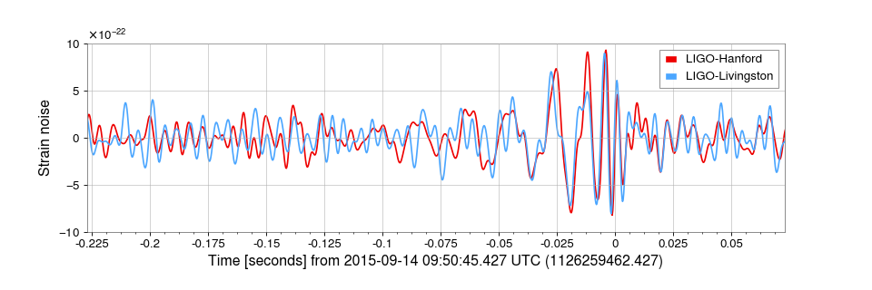
creating a (almost) publication-ready figure of real GW observatory data in just 18 lines of code.