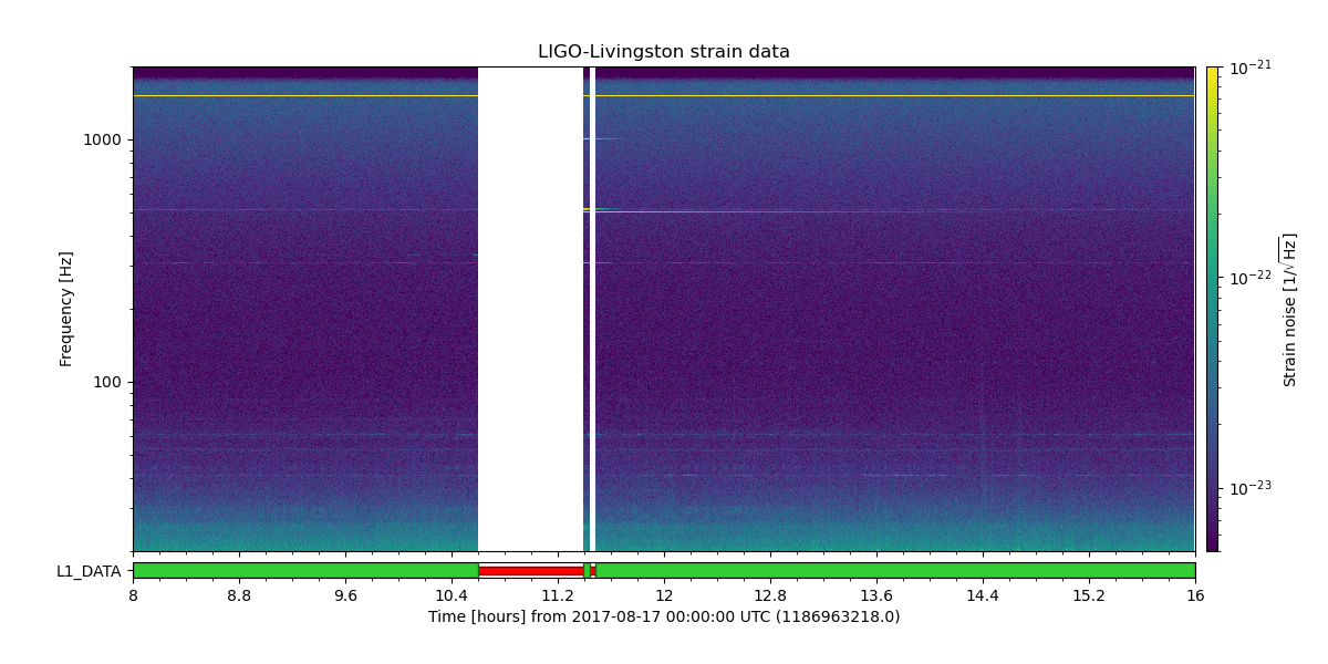
Plotting a spectrogram of all open data for many hours

In order to study interferometer performance, it is common in LIGO to plot all of the data for a day, in order to determine trends, and see data-quality issues.

This is done for the LIGO-Virgo detector network, with up-to-date plots available from GWOSC.

This example demonstrates how to download data segments from GWOSC, then use those to build a multi-hour spectrogram plot of LIGO-Livingston strain data.

Getting the segments

First, we need to fetch the Open Data timeline segments from GWOSC. To do that we can call the DataQualityFlag.fetch_open_data() method using 'H1_DATA' as the flag (for an explanation of what this means, read up on The S6 Data Release).

from gwpy.segments import DataQualityFlag
l1segs = DataQualityFlag.fetch_open_data(
    "L1_DATA",
    "Aug 17 2017 08:00",
    "Aug 17 2017 16:00",
)

For sanity, lets plot these segments:

splot = l1segs.plot(
    figsize=[12, 3],
    epoch="August 17 2017",
)
splot.show()
splot.close()  # hide

We see that the LIGO Hanford Observatory detector was operating for the majority of the day, with a few outages of ~30 minutes or so.

We can use the abs() function to display the total amount of time spent taking data:

print(abs(l1segs.active))

25796

Working with strain data

Now, we can loop through the active segments of 'L1_DATA' and fetch the strain TimeSeries for each segment, calculating a Spectrogram for each segment.

from gwpy.timeseries import TimeSeries
spectrograms = []
for start, end in l1segs.active:
    l1strain = TimeSeries.fetch_open_data(
        "L1",
        start,
        end,
        verbose=True,
    )
    specgram = l1strain.spectrogram(30, fftlength=4) ** (1/2.)
    spectrograms.append(specgram)

Fetched 4 URLs from gwosc.org for [1186992018 .. 1187001382))
Reading data... [Done]
Reading data... [Done]
Reading data... [Done]
Reading data... [Done]
Fetched 1 URLs from gwosc.org for [1187004231 .. 1187004416))
Reading data... [Done]
Fetched 5 URLs from gwosc.org for [1187004571 .. 1187020818))
Reading data... [Done]
Reading data... [Done]
Reading data... [Done]
Reading data... [Done]
Reading data... [Done]

Finally, we can build a plot():

# Create an empty plot with a single set of Axes
from gwpy.plot import Plot
plot = Plot(figsize=(12, 6))
ax = plot.gca()
# add each spectrogram to the Axes
for specgram in spectrograms:
    ax.imshow(specgram)
# finalise the plot metadata
ax.set_xscale("auto-gps", epoch="Aug 17 2017")
ax.set_ylim(20, 2000)
ax.set_yscale("log")
ax.set_ylabel("Frequency [Hz]")
ax.set_title("LIGO-Livingston strain data")
ax.colorbar(
    cmap="viridis",
    norm="log",
    clim=(5e-24, 1e-21),
    label=r"Strain noise [1/$\sqrt{\mathrm{Hz}}$]",
)
# add the segments as a 'state' indicator along the bottom
plot.add_segments_bar(l1segs)
plot.show()