6. Plotting a Rayleigh-statistic Spectrum¶

In LIGO the ‘Rayleigh’ statistic is a calculation of the coefficient of variation of the power spectral density (PSD) of a given set of data. It is used to measure the ‘Gaussianity’ of those data, where a value of 1 indicates Gaussian behaviour, less than 1 indicates coherent variations, and greater than 1 indicates incoherent variation. It is a useful measure of the quality of the strain data being generated and recorded at a LIGO site.

To demonstate this, we can load some data from the LIGO Livingston interferometer around the time of the GW151226 gravitational wave detection:

from gwpy.timeseries import TimeSeries
gwdata = TimeSeries.fetch_open_data("L1", "Dec 26 2015 03:37",
                                    "Dec 26 2015 03:47", verbose=True)

Next, we can calculate a Rayleigh statistic FrequencySeries using the rayleigh_spectrum() method of the TimeSeries with a 2-second FFT and 1-second overlap (50%):

rayleigh = gwdata.rayleigh_spectrum(2, 1)

For easy comparison, we can calculate the spectral sensitivity ASD of the strain data and plot both on the same figure:

from gwpy.plot import Plot
plot = Plot(gwdata.asd(2, 1), rayleigh, geometry=(2, 1), sharex=True,
            xscale="log", xlim=(30, 1500))
asdax, rayax = plot.axes
asdax.set_yscale("log")
asdax.set_ylim(5e-24, 1e-21)
asdax.set_ylabel(r"[strain/$\sqrt{\mathrm{Hz}}$]")
rayax.set_ylim(0, 2)
rayax.set_ylabel("Rayleigh statistic")
asdax.set_title("Sensitivity of LIGO-Livingston around GW151226", fontsize=20)
plot.show()

(png)

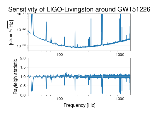
So, we see sharp dips at certain frequencies associated with ‘lines’ in spectrum where noise at a fixed frequency is very coherent (e.g. harmonics of the 60Hz mains power supply), and bumps in specific frequency bands where the interferometer noise is non-stationary.