Note
Go to the end to download the full example code.
Generate the Q-transform of a TimeSeries
One of the most useful tools for filtering and visualising short-duration
features in a TimeSeries is the
Q-transform.
This is regularly used by the Detector Characterization working groups of
the LIGO Scientific Collaboration and the Virgo Collaboration to produce
high-resolution time-frequency maps of transient noise (glitches) and
potential gravitational-wave signals.
This algorithm was used to visualise the first ever gravitational-wave detection GW150914, so we can reproduce that result (bottom panel of figure 1) here.
First, we need to download the TimeSeries record for the H1 strain
measurement from GWOSC:
from gwpy.timeseries import TimeSeries
data = TimeSeries.fetch_open_data("H1", 1126259446, 1126259478)
Next, we generate the q_transform of these data:
qspecgram = data.q_transform(outseg=(1126259462.2, 1126259462.5))
Note
We can save memory by focusing on a specific window around the
interesting time. The outseg keyword argument returns a Spectrogram
that is only as long as we need it to be.
Now, we can plot the resulting Spectrogram:
plot = qspecgram.plot(figsize=[8, 4])
ax = plot.gca()
ax.set_xscale("seconds")
ax.set_yscale("log")
ax.set_ylim(20, 500)
ax.set_ylabel("Frequency [Hz]")
ax.grid(True, axis="y", which="both")
ax.colorbar(cmap="viridis", label="Normalized energy")
plot.show()
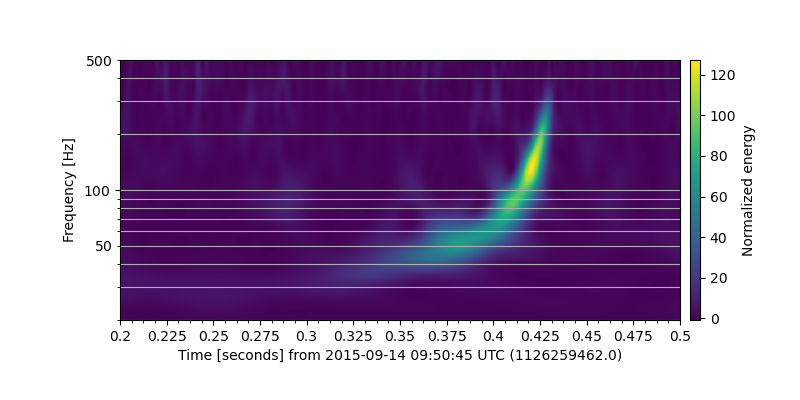
Here we can clearly see the trace of a compact binary coalescence, specifically a binary black hole merger! For more details on this historic result, please see GW150914.
Total running time of the script: (0 minutes 2.324 seconds)