Command line plotting with GWpy
LigoDV-web (https://ldvw.ligo.caltech.edu) is a web based tool for viewing LIGO data. With the availability of GWpy we have undergone a transformation from using our own plotting functions to using GWpy. Since ldvw is written in Java the most effective way to do this was to develop a command line program to generate each of the plots. This program is now part of the GWpy distribution and can be used on any machine with GWpy installed including Condor compute nodes.
The general form of the command is:
gwpy-plot ACTION REQUIRED-ARGUMENTS or --help [OPTIONS]
Where ACTION is the name of the plot to make. If you run the script without any agruments it will list the actions.
$ gwpy-plot
usage: gwpy-plot [-h]
                 {timeseries,coherence,spectrum,spectrogram,coherencegram} ...
gwpy-plot: error: too few arguments
To see the available options for any action add the action keyword. For example:
$ gwpy-plot timeseries
usage: gwpy-plot timeseries [-h] [-v] [-s SILENT] --chan CHAN [CHAN ...]
                            --start START [START ...] [--duration DURATION]
                            [-c FRAMECACHE] [--highpass HIGHPASS] [--logx]
                            [--xmin XMIN] [--xmax XMAX] [-g GEOMETRY]
                            [--interactive] [--logy] [--title TITLE]
                            [--suptitle SUPTITLE] [--xlabel XLABEL]
                            [--ylabel YLABEL] [--out OUT]
                            [--legend [LEGEND [LEGEND ...]]] [--nolegend]
                            [--nogrid] [--ymin YMIN] [--ymax YMAX]
A -h or --help after the action will provide an explanation of each option. Since most
options are shared among several actions we will discuss them in groups.
The program tries to choose reasonable defaults so the only required arguments for most plots are one channel and one start time, some plots like coherence require two channels. For example:
gwpy-plot timeseries --chan L1:OAF-CAL_DARM_DQ --start 1102766651
Will produce a image file called gwpy.png in the current directory that looks like:
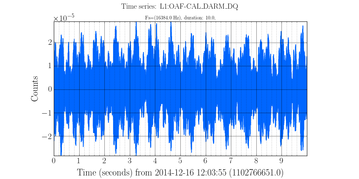
To generate that image several assumptions were made such as using 10 sec of data from a default NDS2 server, scaling the plot to the full range on both X and Y axes, using standard labeling and output went to a generic file in the current directory. All of this is customizable, plus we can use log scaling or high pass filter the data before plotting.
The options for each action vary but many are common.
Specify input data
The line plots: time series, spectrum, and coherence accept multiple channels and multiple times, while the image plots: spectrogram and coherence-spectrogram accept only one (spectrogram) or two (coherence-spectrogram) channel(s) and one time.
Channels are specified using their full name and it is case sensitive.
Use the --chan argument followed by the channel name as many times as needed
Start times are specified in GPS seconds. Use the --start argument followed by the start time
as many times as needed.
Duration is specified in seconds using the --duration keyword. There is only
one duration and it applies to all channels and all start times.
By default all data is pulled from an appropriate NDS2 server using GWpy’s algorithm to decide which
servers to try, in what order. You can use the -c or --framecache argument to
specify a LAL style frame cache if you prefer to get the data from .gwf frame files.
Prefiltering data
Data may be high pass filtered with a Butterworth window before any processing or plotting is done.
The --highpass <cutoff frequency (Hz)> pair specifies the filter.
Titles, lables, and legends
The figure below is a spectrum that was generated with the command line:
gwpy-plot spectrum --chan L1:OAF-CAL_DARM_DQ --start 1102766451 1102766651 --out spectrum.png
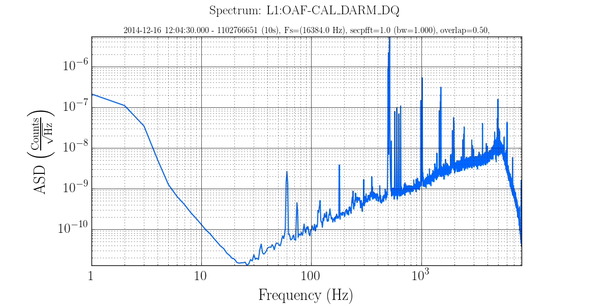
The top line is called the super title and is overridden with the --suptitle directive followed
by the new supertitle which may be plain text or LaTex. There can be only 1 supertitle and it is one
line only. Be sure to put quotes (” or ‘) around any string with spaces or special characters.
The line below that is called the title and is overridden with the --title directive followed by
the new title. There can be multiple titles limited only by space available on the image.
The X-axis and the Y-axis labels are set with the --xlabel and -ylabel argument.
The legends only appear by default when more than one dataset is plotted. The text for each legend
can be set with the --legend argument, one for each dataset. The --nolegend argument turns
off all legends.
The gridlines are shown by default. To remove them from the plot use the --nogrid argument.
Interactive mode
The --interactive argument uses the matplotlib/pyplot show function to display an image and allow
simple manipulations such as zoom, pan, and comfigure subplots. There is also a save function. gwpy-plot
will also save the image generated. Interactive mode is described in detail in the Interactive mode
section.
Customizing individual plots
Individual plots may have different default behavior and different arguments. This section discussed options that behave the same for all plots. See the appropriate section below for the remainder of the arguments for each plot.