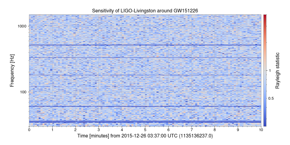
5. Plotting a Spectrogram of the Rayleigh statistic
As described in Plotting a Rayleigh-statistic Spectrum, the Rayleigh statistic can be used to study non-Gaussianity in a timeseries. We can study the time variance of these features by plotting a time-frequency spectrogram where we calculate the Rayleigh statistic for each time bin.
To demonstate this, we can load some data from the LIGO Livingston intereferometer around the time of the GW151226 gravitational wave detection:
from gwpy.timeseries import TimeSeries
gwdata = TimeSeries.fetch_open_data('L1', 'Dec 26 2015 03:37',
                                    'Dec 26 2015 03:47', verbose=True)
Next, we can calculate a Rayleigh statistic Spectrogram using the
rayleigh_spectrogram() method of the
TimeSeries and a 5-second stride with a 2-second FFT and
1-second overlap (50%):
rayleigh = gwdata.rayleigh_spectrogram(5, fftlength=2, overlap=1)
and can make a plot using the plot() method
plot = rayleigh.plot(norm='log', vmin=0.25, vmax=4)
ax = plot.gca()
ax.set_yscale('log')
ax.set_ylim(30, 1500)
ax.set_title('Sensitivity of LIGO-Livingston around GW151226')
ax.colorbar(cmap='coolwarm', label='Rayleigh statistic')
plot.show()
(png)
