Plotting time-domain data¶

Plotting one TimeSeries¶

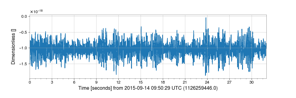
The TimeSeries class includes a plot() method to trivialise visualisation of the contained data. Reproducing the example from gwpy-timeseries-remote:

>>> l1hoft = TimeSeries.fetch_open_data('L1', 'Sep 14 2015 09:50:29', 'Sep 14 2015 09:51:01')
>>> plot = l1hoft.plot()
>>> plot.show()

(png)

The returned object plot is a Plot, a sub-class of matplotlib.figure.Figure adapted for GPS time-stamped data. Customisations of the figure or the underlying Axes can be done using standard matplotlib methods. For example:

>>> ax = plot.gca()
>>> ax.set_ylabel('Gravitational-wave amplitude [strain]')
>>> ax.set_epoch(1126259462)
>>> ax.set_title('LIGO-Livingston strain data around GW150914')
>>> ax.axvline(1126259462, color='orange', linestyle='--')
>>> plot.refresh()

(png)

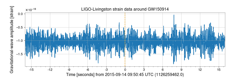
Here the set_epoch() method is used to reset the reference time for the x-axis.

Plotting multiple TimeSeries together¶

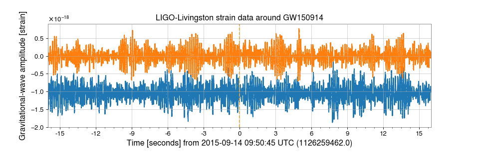
Multiple TimeSeries classes can be combined on a figure in a number of different ways, the most obvious is to plot() the first, then add the second on the same axes. Reusing the same plot from above:

>>> h1hoft = TimeSeries.fetch_open_data('H1', 'Sep 14 2015 09:50:29', 'Sep 14 2015 09:51:01')
>>> ax = plot.gca()
>>> ax.plot(h1hoft)
>>> plot.refresh()

(png)

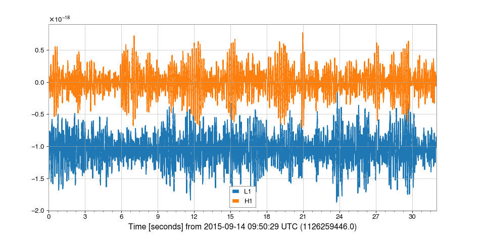
Alternatively, the two TimeSeries could be combined into a TimeSeriesDict to use the plot() method from that class:

>>> combined = TimeSeriesDict()
>>> combined['L1'] = l1hoft
>>> combined['H1'] = h1hoft
>>> plot = combined.plot()
>>> plot.gca().legend()
>>> plot.show()

(png)

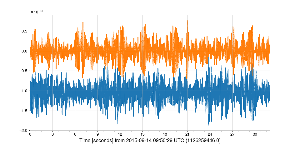
The third method of achieving the same result is by importing and accessing the Plot object directly:

>>> from gwpy.plot import Plot
>>> plot = Plot(l1hoft, h1hoft)
>>> plot.show()

(png)

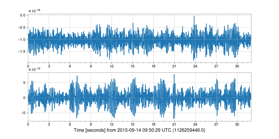
Using the Plot directly allows for greater customisation. The separate=True keyword argument can be used to plot each TimeSeries on its own axes, with sharex=True given to link the time scales for each Axes:

>>> plot = Plot(l1hoft, h1hoft, separate=True, sharex=True)
>>> plot.show()

(png)