TimeSeries
-
class gwpy.timeseries.TimeSeries(data, unit=
None, t0=None, dt=None, sample_rate=None, times=None, channel=None, name=None, **kwargs)[source]¶ A time-domain data array.
- Parameters:
- valuearray-like
input data array
- unit
Unit, optional physical unit of these data
- t0
LIGOTimeGPS,float,str, optional GPS epoch associated with these data, any input parsable by
to_gpsis fine- dt
float,Quantity, optional time between successive samples (seconds), can also be given inversely via
sample_rate- sample_rate
float,Quantity, optional the rate of samples per second (Hertz), can also be given inversely via
dt- times
array-like the complete array of GPS times accompanying the data for this series. This argument takes precedence over
t0anddtso should be given in place of these if relevant, not alongside- name
str, optional descriptive title for this array
- channel
Channel,str, optional source data stream for these data
- dtype
dtype, optional input data type
- copy
bool, optional choose to copy the input data to new memory
- subok
bool, optional allow passing of sub-classes by the array generator
Notes
The necessary metadata to reconstruct timing information are recorded in the
epochandsample_rateattributes. This time-stamps can be returned via thetimesproperty.All comparison operations performed on a
TimeSerieswill return aStateTimeSeries- a boolean array with metadata copied from the startingTimeSeries.Examples
>>> from gwpy.timeseries import TimeSeriesTo create an array of random numbers, sampled at 100 Hz, in units of ‘metres’:
>>> from numpy import random
>>> series = TimeSeries(random.random(1000), sample_rate=100, unit='m')
which can then be simply visualised via
>>> plot = series.plot()
>>> plot.show()
(
png)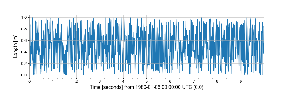
Attributes Summary
View of the transposed array.
Base object if memory is from some other object.
Returns a copy of the current
Quantityinstance with CGS units.Instrumental channel associated with these data
An object to simplify the interaction of the array with the ctypes module.
Python buffer object pointing to the start of the array's data.
X-axis sample separation
Data-type of the array's elements.
Duration of this series in seconds
X-axis sample separation
GPS epoch for these data.
A list of equivalencies that will be applied by default during unit conversions.
Information about the memory layout of the array.
A 1-D iterator over the Quantity array.
The imaginary part of the array.
Container for meta information like name, description, format.
True if the
valueof this quantity is a scalar, or False if it is an array-like object.Length of one array element in bytes.
View of the matrix transposed array.
Name for this data set
Total bytes consumed by the elements of the array.
Number of array dimensions.
The real part of the array.
Data rate for this
TimeSeriesin samples per second (Hertz).Tuple of array dimensions.
Returns a copy of the current
Quantityinstance with SI units.Number of elements in the array.
X-axis [low, high) segment encompassed by these data
Tuple of bytes to step in each dimension when traversing an array.
X-axis coordinate of the first data point
Positions of the data on the x-axis
The physical unit of these data
The numerical value of this instance.
X-axis coordinate of the first data point
Positions of the data on the x-axis
X-axis [low, high) segment encompassed by these data
Unit of x-axis index
Methods Summary
abs(x, /[, out, where, casting, order, ...])Calculate the absolute value element-wise.
all([axis, out, keepdims, where])Returns True if all elements evaluate to True.
any([axis, out, keepdims, where])Returns True if any of the elements of
aevaluate to True.append(other[, inplace, pad, gap, resize])Connect another series onto the end of the current one.
argmax([axis, out, keepdims])Return indices of the maximum values along the given axis.
argmin([axis, out, keepdims])Return indices of the minimum values along the given axis.
argpartition(kth[, axis, kind, order])Returns the indices that would partition this array.
argsort([axis, kind, order])Returns the indices that would sort this array.
asd([fftlength, overlap, window, method])Calculate the ASD
FrequencySeriesof thisTimeSeriesastype(dtype[, order, casting, subok, copy])Copy of the array, cast to a specified type.
auto_coherence(dt[, fftlength, overlap, window])Calculate the frequency-coherence between this
TimeSeriesand a time-shifted copy of itself.average_fft([fftlength, overlap, window])Compute the averaged one-dimensional DFT of this
TimeSeries.bandpass(flow, fhigh[, gpass, gstop, fstop, ...])Filter this
TimeSerieswith a band-pass filter.byteswap([inplace])Swap the bytes of the array elements
choose(choices[, out, mode])Use an index array to construct a new array from a set of choices.
clip([min, max, out])Return an array whose values are limited to
[min, max].coherence(other[, fftlength, overlap, window])Calculate the frequency-coherence between this
TimeSeriesand another.coherence_spectrogram(other, stride[, ...])Calculate the coherence spectrogram between this
TimeSeriesand other.compress(condition[, axis, out])Return selected slices of this array along given axis.
conj()Complex-conjugate all elements.
Return the complex conjugate, element-wise.
convolve(fir[, window])Convolve this
TimeSerieswith an FIR filter using thecopy([order])Return a copy of the array.
correlate(mfilter[, window, detrend, ...])Cross-correlate this
TimeSerieswith another signalcrop([start, end, copy])Crop this series to the given x-axis extent.
csd(other[, fftlength, overlap, window])Calculate the CSD
FrequencySeriesfor twoTimeSeriescsd_spectrogram(other, stride[, fftlength, ...])Calculate the cross spectral density spectrogram of this
cumprod([axis, dtype, out])Return the cumulative product of the elements along the given axis.
cumsum([axis, dtype, out])Return the cumulative sum of the elements along the given axis.
decompose([bases])Generates a new
Quantitywith the units decomposed.demodulate(f[, stride, exp, deg])Compute the average magnitude and phase of this
TimeSeriesonce per stride at a given frequencydetrend([detrend])Remove the trend from this
TimeSeriesdiagonal([offset, axis1, axis2])Return specified diagonals.
diff([n, axis])Calculate the n-th order discrete difference along given axis.
dot(b[, out])dump(file)Not implemented, use
.value.dump()instead.dumps()Returns the pickle of the array as a string.
ediff1d([to_end, to_begin])fetch(channel, start, end[, host, port, ...])Fetch data from NDS
fetch_open_data(ifo, start, end[, ...])Fetch open-access data from the LIGO Open Science Center
fft([nfft])Compute the one-dimensional discrete Fourier transform of this
TimeSeries.fftgram(fftlength[, overlap, window])Calculate the Fourier-gram of this
TimeSeries.fill(value)Fill the array with a scalar value.
filter(*filt, **kwargs)Filter this
TimeSerieswith an IIR or FIR filterfind(channel, start, end[, frametype, pad, ...])Find and read data from frames for a channel
find_gates([tzero, whiten, threshold, ...])Identify points that should be gates using a provided threshold and clustered within a provided time window.
flatten([order])Return a copy of the array collapsed into one dimension.
from_lal(lalts[, copy])Generate a new TimeSeries from a LAL TimeSeries of any type.
from_nds2_buffer(buffer_[, scaled, copy])Construct a new series from an
nds2.bufferobjectfrom_pycbc(pycbcseries[, copy])Convert a
pycbc.types.timeseries.TimeSeriesinto aTimeSeriesgate([tzero, tpad, whiten, threshold, ...])Removes high amplitude peaks from data using inverse Planck window.
get(channel, start, end[, pad, scaled, ...])Get data for this channel from frames or NDS
getfield(dtype[, offset])Returns a field of the given array as a certain type.
heterodyne(phase[, stride, singlesided])Compute the average magnitude and phase of this
TimeSeriesonce per stride after heterodyning with a given phase serieshighpass(frequency[, gpass, gstop, fstop, ...])Filter this
TimeSerieswith a high-pass filter.inject(other)Add two compatible
Seriesalong their shared x-axis values.insert(obj, values[, axis])Insert values along the given axis before the given indices and return a new
Quantityobject.is_compatible(other)Check whether this series and other have compatible metadata
is_contiguous(other[, tol])Check whether other is contiguous with self.
item(*args)Copy an element of an array to a scalar Quantity and return it.
lowpass(frequency[, gpass, gstop, fstop, ...])Filter this
TimeSerieswith a Butterworth low-pass filter.mask([deadtime, flag, query_open_data, ...])Mask away portions of this
TimeSeriesthat fall within a given list of time segmentsmax([axis, out, keepdims, initial, where])Return the maximum along a given axis.
mean([axis, dtype, out, keepdims, where])Returns the average of the array elements along given axis.
median([axis])Compute the median along the specified axis.
min([axis, out, keepdims, initial, where])Return the minimum along a given axis.
nonzero()Return the indices of the elements that are non-zero.
notch(frequency[, type, filtfilt])Notch out a frequency in this
TimeSeries.override_unit(unit[, parse_strict])Forcefully reset the unit of these data
pad(pad_width, **kwargs)Pad this series to a new size
partition(kth[, axis, kind, order])Partially sorts the elements in the array in such a way that the value of the element in k-th position is in the position it would be in a sorted array.
plot([method, figsize, xscale])Plot the data for this timeseries
prepend(other[, inplace, pad, gap, resize])Connect another series onto the start of the current one.
prod([axis, dtype, out, keepdims, initial, ...])Return the product of the array elements over the given axis
psd([fftlength, overlap, window, method])Calculate the PSD
FrequencySeriesfor thisTimeSeriesput(indices, values[, mode])Set
a.flat[n] = values[n]for allnin indices.q_gram([qrange, frange, mismatch, snrthresh])Scan a
TimeSeriesusing the multi-Q transform and return anEventTableof the most significant tilesq_transform([qrange, frange, gps, search, ...])Scan a
TimeSeriesusing the multi-Q transform and return an interpolated high-resolution spectrogramravel([order])Return a flattened array.
rayleigh_spectrogram(stride[, fftlength, ...])Calculate the Rayleigh statistic spectrogram of this
TimeSeriesrayleigh_spectrum([fftlength, overlap, window])Calculate the Rayleigh
FrequencySeriesfor thisTimeSeries.read(source, *args, **kwargs)Read data into a
TimeSeriesrepeat(repeats[, axis])Repeat elements of an array.
resample(rate[, window, ftype, n])Resample this Series to a new rate
reshape(shape, /, *[, order, copy])Returns an array containing the same data with a new shape.
resize(new_shape[, refcheck])Change shape and size of array in-place.
rms([stride])Calculate the root-mean-square value of this
TimeSeriesonce per stride.round([decimals, out])Return
awith each element rounded to the given number of decimals.searchsorted(v[, side, sorter])Find indices where elements of v should be inserted in a to maintain order.
setfield(val, dtype[, offset])Put a value into a specified place in a field defined by a data-type.
setflags([write, align, uic])Set array flags WRITEABLE, ALIGNED, WRITEBACKIFCOPY, respectively.
shift(delta)Shift this
Seriesforward on the X-axis bydeltasort([axis, kind, order])Sort an array in-place.
spectral_variance(stride[, fftlength, ...])Calculate the
SpectralVarianceof thisTimeSeries.spectrogram(stride[, fftlength, overlap, ...])Calculate the average power spectrogram of this
TimeSeriesusing the specified average spectrum method.spectrogram2(fftlength[, overlap, window])Calculate the non-averaged power
Spectrogramof thisTimeSeriessqueeze([axis])Remove axes of length one from
a.std([axis, dtype, out, ddof, keepdims, where])Returns the standard deviation of the array elements along given axis.
step(**kwargs)Create a step plot of this series
sum([axis, dtype, out, keepdims, initial, where])Return the sum of the array elements over the given axis.
swapaxes(axis1, axis2)Return a view of the array with
axis1andaxis2interchanged.take(indices[, axis, out, mode])Return an array formed from the elements of
aat the given indices.taper([side, duration, nsamples])Taper the ends of this
TimeSeriessmoothly to zero.to(unit[, equivalencies, copy])Return a new
Quantityobject with the specified unit.to_lal()Convert this
TimeSeriesinto a LAL TimeSeries.to_pycbc([copy])Convert this
TimeSeriesinto a PyCBCTimeSeriesto_string([unit, precision, format, subfmt, ...])Generate a string representation of the quantity and its unit.
to_value([unit, equivalencies])The numerical value, possibly in a different unit.
tobytes([order])Not implemented, use
.value.tobytes()instead.tofile(fid[, sep, format])Not implemented, use
.value.tofile()instead.tolist()Return the array as an
a.ndim-levels deep nested list of Python scalars.tostring([order])Construct Python bytes containing the raw data bytes in the array.
trace([offset, axis1, axis2, dtype, out])Return the sum along diagonals of the array.
transfer_function(other[, fftlength, ...])Calculate the transfer function between this
TimeSeriesand another.transpose(*axes)Returns a view of the array with axes transposed.
update(other[, inplace])Update this series by appending new data from an other and dropping the same amount of data off the start.
value_at(x)Return the value of this
Seriesat the givenxindexvaluevar([axis, dtype, out, ddof, keepdims, where])Returns the variance of the array elements, along given axis.
view([dtype][, type])New view of array with the same data.
whiten([fftlength, overlap, method, window, ...])Whiten this
TimeSeriesusing inverse spectrum truncationwrite(target, *args, **kwargs)Write this
TimeSeriesto a filezip()zpk(zeros, poles, gain[, analog])Filter this
TimeSeriesby applying a zero-pole-gain filterAttributes Documentation
- T
View of the transposed array.
Same as
self.transpose().See also
Examples
>>> import numpy as np
>>> a = np.array([[1, 2], [3, 4]])
>>> a
array([[1, 2],
       [3, 4]])
>>> a.T
array([[1, 3],
       [2, 4]])
>>> a = np.array([1, 2, 3, 4]) >>> a array([1, 2, 3, 4]) >>> a.T array([1, 2, 3, 4])
- base
Base object if memory is from some other object.
Examples
The base of an array that owns its memory is None:
>>> import numpy as np
>>> x = np.array([1,2,3,4])
>>> x.base is None
True
Slicing creates a view, whose memory is shared with x:
>>> y = x[2:]
>>> y.base is x
True
- cgs
Returns a copy of the current
Quantityinstance with CGS units. The value of the resulting object will be scaled.
- ctypes
An object to simplify the interaction of the array with the ctypes module.
This attribute creates an object that makes it easier to use arrays when calling shared libraries with the ctypes module. The returned object has, among others, data, shape, and strides attributes (see Notes below) which themselves return ctypes objects that can be used as arguments to a shared library.
See also
Notes
Below are the public attributes of this object which were documented in “Guide to NumPy” (we have omitted undocumented public attributes, as well as documented private attributes):
- _ctypes.data
A pointer to the memory area of the array as a Python integer. This memory area may contain data that is not aligned, or not in correct byte-order. The memory area may not even be writeable. The array flags and data-type of this array should be respected when passing this attribute to arbitrary C-code to avoid trouble that can include Python crashing. User Beware! The value of this attribute is exactly the same as:
self._array_interface_['data'][0].Note that unlike
data_as, a reference won’t be kept to the array: code likectypes.c_void_p((a + b).ctypes.data)will result in a pointer to a deallocated array, and should be spelt(a + b).ctypes.data_as(ctypes.c_void_p)
- _ctypes.shape
(c_intp*self.ndim): A ctypes array of length self.ndim where the basetype is the C-integer corresponding to
dtype('p')on this platform (seec_intp). This base-type could bectypes.c_int,ctypes.c_long, orctypes.c_longlongdepending on the platform. The ctypes array contains the shape of the underlying array.
- _ctypes.strides
(c_intp*self.ndim): A ctypes array of length self.ndim where the basetype is the same as for the shape attribute. This ctypes array contains the strides information from the underlying array. This strides information is important for showing how many bytes must be jumped to get to the next element in the array.
- _ctypes.data_as(obj)
Return the data pointer cast to a particular c-types object. For example, calling
self._as_parameter_is equivalent toself.data_as(ctypes.c_void_p). Perhaps you want to use the data as a pointer to a ctypes array of floating-point data:self.data_as(ctypes.POINTER(ctypes.c_double)).The returned pointer will keep a reference to the array.
- _ctypes.shape_as(obj)
Return the shape tuple as an array of some other c-types type. For example:
self.shape_as(ctypes.c_short).
- _ctypes.strides_as(obj)
Return the strides tuple as an array of some other c-types type. For example:
self.strides_as(ctypes.c_longlong).
If the ctypes module is not available, then the ctypes attribute of array objects still returns something useful, but ctypes objects are not returned and errors may be raised instead. In particular, the object will still have the
as_parameterattribute which will return an integer equal to the data attribute.Examples
>>> import numpy as np
>>> import ctypes
>>> x = np.array([[0, 1], [2, 3]], dtype=np.int32)
>>> x
array([[0, 1],
       [2, 3]], dtype=int32)
>>> x.ctypes.data
31962608 # may vary
>>> x.ctypes.data_as(ctypes.POINTER(ctypes.c_uint32))
<__main__.LP_c_uint object at 0x7ff2fc1fc200> # may vary
>>> x.ctypes.data_as(ctypes.POINTER(ctypes.c_uint32)).contents
c_uint(0)
>>> x.ctypes.data_as(ctypes.POINTER(ctypes.c_uint64)).contents
c_ulong(4294967296)
>>> x.ctypes.shape
<numpy._core._internal.c_long_Array_2 object at 0x7ff2fc1fce60> # may vary
>>> x.ctypes.strides
<numpy._core._internal.c_long_Array_2 object at 0x7ff2fc1ff320> # may vary
- data
Python buffer object pointing to the start of the array’s data.
- device
- dtype
Data-type of the array’s elements.
Warning
Setting
arr.dtypeis discouraged and may be deprecated in the future. Setting will replace thedtypewithout modifying the memory (see alsondarray.viewandndarray.astype).See also
ndarray.astypeCast the values contained in the array to a new data-type.
ndarray.viewCreate a view of the same data but a different data-type.
numpy.dtype
Examples
>>> x
array([[0, 1],
       [2, 3]])
>>> x.dtype
dtype('int32')
>>> type(x.dtype)
<type 'numpy.dtype'>
- equivalencies
A list of equivalencies that will be applied by default during unit conversions.
- flags
Information about the memory layout of the array.
- Attributes:
- C_CONTIGUOUS (C)
The data is in a single, C-style contiguous segment.
- F_CONTIGUOUS (F)
The data is in a single, Fortran-style contiguous segment.
- OWNDATA (O)
The array owns the memory it uses or borrows it from another object.
- WRITEABLE (W)
The data area can be written to. Setting this to False locks the data, making it read-only. A view (slice, etc.) inherits WRITEABLE from its base array at creation time, but a view of a writeable array may be subsequently locked while the base array remains writeable. (The opposite is not true, in that a view of a locked array may not be made writeable. However, currently, locking a base object does not lock any views that already reference it, so under that circumstance it is possible to alter the contents of a locked array via a previously created writeable view onto it.) Attempting to change a non-writeable array raises a RuntimeError exception.
- ALIGNED (A)
The data and all elements are aligned appropriately for the hardware.
- WRITEBACKIFCOPY (X)
This array is a copy of some other array. The C-API function PyArray_ResolveWritebackIfCopy must be called before deallocating to the base array will be updated with the contents of this array.
- FNC
F_CONTIGUOUS and not C_CONTIGUOUS.
- FORC
F_CONTIGUOUS or C_CONTIGUOUS (one-segment test).
- BEHAVED (B)
ALIGNED and WRITEABLE.
- CARRAY (CA)
BEHAVED and C_CONTIGUOUS.
- FARRAY (FA)
BEHAVED and F_CONTIGUOUS and not C_CONTIGUOUS.
Notes
The
flagsobject can be accessed dictionary-like (as ina.flags['WRITEABLE']), or by using lowercased attribute names (as ina.flags.writeable). Short flag names are only supported in dictionary access.Only the WRITEBACKIFCOPY, WRITEABLE, and ALIGNED flags can be changed by the user, via direct assignment to the attribute or dictionary entry, or by calling
ndarray.setflags.The array flags cannot be set arbitrarily:
WRITEBACKIFCOPY can only be set
False.ALIGNED can only be set
Trueif the data is truly aligned.WRITEABLE can only be set
Trueif the array owns its own memory or the ultimate owner of the memory exposes a writeable buffer interface or is a string.
Arrays can be both C-style and Fortran-style contiguous simultaneously. This is clear for 1-dimensional arrays, but can also be true for higher dimensional arrays.
Even for contiguous arrays a stride for a given dimension
arr.strides[dim]may be arbitrary ifarr.shape[dim] == 1or the array has no elements. It does not generally hold thatself.strides[-1] == self.itemsizefor C-style contiguous arrays orself.strides[0] == self.itemsizefor Fortran-style contiguous arrays is true.
- flat
A 1-D iterator over the Quantity array.
This returns a
QuantityIteratorinstance, which behaves the same as theflatiterinstance returned byflat, and is similar to, but not a subclass of, Python’s built-in iterator object.
- imag
The imaginary part of the array.
Examples
>>> import numpy as np
>>> x = np.sqrt([1+0j, 0+1j])
>>> x.imag
array([ 0.        ,  0.70710678])
>>> x.imag.dtype
dtype('float64')
- info
Container for meta information like name, description, format. This is required when the object is used as a mixin column within a table, but can be used as a general way to store meta information.
- isscalar
True if the
valueof this quantity is a scalar, or False if it is an array-like object.Note
This is subtly different from
numpy.isscalarin thatnumpy.isscalarreturns False for a zero-dimensional array (e.g.np.array(1)), while this is True for quantities, since quantities cannot represent true numpy scalars.
- itemset
- itemsize
Length of one array element in bytes.
Examples
>>> import numpy as np
>>> x = np.array([1,2,3], dtype=np.float64)
>>> x.itemsize
8
>>> x = np.array([1,2,3], dtype=np.complex128)
>>> x.itemsize
16
- mT
View of the matrix transposed array.
The matrix transpose is the transpose of the last two dimensions, even if the array is of higher dimension.
Added in version 2.0.
- Raises:
- ValueError
If the array is of dimension less than 2.
Examples
>>> import numpy as np
>>> a = np.array([[1, 2], [3, 4]])
>>> a
array([[1, 2],
       [3, 4]])
>>> a.mT
array([[1, 3],
       [2, 4]])
>>> a = np.arange(8).reshape((2, 2, 2)) >>> a array([[[0, 1], [2, 3]], [[4, 5], [6, 7]]]) >>> a.mT array([[[0, 2], [1, 3]], [[4, 6], [5, 7]]])
- nbytes
Total bytes consumed by the elements of the array.
See also
sys.getsizeofMemory consumed by the object itself without parents in case view. This does include memory consumed by non-element attributes.
Notes
Does not include memory consumed by non-element attributes of the array object.
Examples
>>> import numpy as np
>>> x = np.zeros((3,5,2), dtype=np.complex128)
>>> x.nbytes
480
>>> np.prod(x.shape) * x.itemsize
480
- ndim
Number of array dimensions.
Examples
>>> import numpy as np
>>> x = np.array([1, 2, 3])
>>> x.ndim
1
>>> y = np.zeros((2, 3, 4))
>>> y.ndim
3
- newbyteorder
- ptp
- real
The real part of the array.
See also
numpy.realequivalent function
Examples
>>> import numpy as np
>>> x = np.sqrt([1+0j, 0+1j])
>>> x.real
array([ 1.        ,  0.70710678])
>>> x.real.dtype
dtype('float64')
- sample_rate
Data rate for this
TimeSeriesin samples per second (Hertz).This attribute is stored internally by the
dxattribute
- shape
Tuple of array dimensions.
The shape property is usually used to get the current shape of an array, but may also be used to reshape the array in-place by assigning a tuple of array dimensions to it. As with
numpy.reshape, one of the new shape dimensions can be -1, in which case its value is inferred from the size of the array and the remaining dimensions. Reshaping an array in-place will fail if a copy is required.Warning
Setting
arr.shapeis discouraged and may be deprecated in the future. Usingndarray.reshapeis the preferred approach.See also
numpy.shapeEquivalent getter function.
numpy.reshapeFunction similar to setting
shape.ndarray.reshapeMethod similar to setting
shape.
Examples
>>> import numpy as np
>>> x = np.array([1, 2, 3, 4])
>>> x.shape
(4,)
>>> y = np.zeros((2, 3, 4))
>>> y.shape
(2, 3, 4)
>>> y.shape = (3, 8)
>>> y
array([[ 0.,  0.,  0.,  0.,  0.,  0.,  0.,  0.],
       [ 0.,  0.,  0.,  0.,  0.,  0.,  0.,  0.],
       [ 0.,  0.,  0.,  0.,  0.,  0.,  0.,  0.]])
>>> y.shape = (3, 6)
Traceback (most recent call last):
  File "<stdin>", line 1, in <module>
ValueError: total size of new array must be unchanged
>>> np.zeros((4,2))[::2].shape = (-1,)
Traceback (most recent call last):
  File "<stdin>", line 1, in <module>
AttributeError: Incompatible shape for in-place modification. Use
`.reshape()` to make a copy with the desired shape.
- si
Returns a copy of the current
Quantityinstance with SI units. The value of the resulting object will be scaled.
- size
Number of elements in the array.
Equal to
np.prod(a.shape), i.e., the product of the array’s dimensions.Notes
a.sizereturns a standard arbitrary precision Python integer. This may not be the case with other methods of obtaining the same value (like the suggestednp.prod(a.shape), which returns an instance ofnp.int_), and may be relevant if the value is used further in calculations that may overflow a fixed size integer type.Examples
>>> import numpy as np
>>> x = np.zeros((3, 5, 2), dtype=np.complex128)
>>> x.size
30
>>> np.prod(x.shape)
30
- strides
Tuple of bytes to step in each dimension when traversing an array.
The byte offset of element
(i[0], i[1], ..., i[n])in an arrayais:offset = sum(np.array(i) * a.strides)A more detailed explanation of strides can be found in The N-dimensional array (ndarray).
Warning
Setting
arr.stridesis discouraged and may be deprecated in the future.numpy.lib.stride_tricks.as_stridedshould be preferred to create a new view of the same data in a safer way.See also
Notes
Imagine an array of 32-bit integers (each 4 bytes):
x = np.array([[0, 1, 2, 3, 4],
              [5, 6, 7, 8, 9]], dtype=np.int32)
This array is stored in memory as 40 bytes, one after the other (known as a contiguous block of memory). The strides of an array tell us how many bytes we have to skip in memory to move to the next position along a certain axis. For example, we have to skip 4 bytes (1 value) to move to the next column, but 20 bytes (5 values) to get to the same position in the next row. As such, the strides for the array
xwill be(20, 4).Examples
>>> import numpy as np
>>> y = np.reshape(np.arange(2*3*4), (2,3,4))
>>> y
array([[[ 0,  1,  2,  3],
        [ 4,  5,  6,  7],
        [ 8,  9, 10, 11]],
       [[12, 13, 14, 15],
        [16, 17, 18, 19],
        [20, 21, 22, 23]]])
>>> y.strides
(48, 16, 4)
>>> y[1,1,1]
17
>>> offset=sum(y.strides * np.array((1,1,1)))
>>> offset/y.itemsize
17
>>> x = np.reshape(np.arange(5*6*7*8), (5,6,7,8)).transpose(2,3,1,0) >>> x.strides (32, 4, 224, 1344) >>> i = np.array([3,5,2,2]) >>> offset = sum(i * x.strides) >>> x[3,5,2,2] 813 >>> offset / x.itemsize 813
- value
The numerical value of this instance.
See also
to_valueGet the numerical value in a given unit.
Methods Documentation
- abs(x, /, out=None, *, where=True, casting='same_kind', order='K', dtype=None, subok=True[, signature])[source]
Calculate the absolute value element-wise.
np.absis a shorthand for this function.- Parameters:
- xarray_like
Input array.
- outndarray, None, or tuple of ndarray and None, optional
A location into which the result is stored. If provided, it must have a shape that the inputs broadcast to. If not provided or None, a freshly-allocated array is returned. A tuple (possible only as a keyword argument) must have length equal to the number of outputs.
- wherearray_like, optional
This condition is broadcast over the input. At locations where the condition is True, the
outarray will be set to the ufunc result. Elsewhere, theoutarray will retain its original value. Note that if an uninitializedoutarray is created via the defaultout=None, locations within it where the condition is False will remain uninitialized.- **kwargs
For other keyword-only arguments, see the ufunc docs.
- Returns:
- absolutendarray
An ndarray containing the absolute value of each element in
x. For complex input,a + ib, the absolute value is . This is a scalar ifxis a scalar.
Examples
>>> import numpy as np
>>> x = np.array([-1.2, 1.2])
>>> np.absolute(x)
array([ 1.2,  1.2])
>>> np.absolute(1.2 + 1j)
1.5620499351813308
Plot the function over
[-10, 10]:>>> import matplotlib.pyplot as plt>>> x = np.linspace(start=-10, stop=10, num=101) >>> plt.plot(x, np.absolute(x)) >>> plt.show()(
png)
Plot the function over the complex plane:
>>> xx = x + 1j * x[:, np.newaxis]
>>> plt.imshow(np.abs(xx), extent=[-10, 10, -10, 10], cmap='gray')
>>> plt.show()
(
png)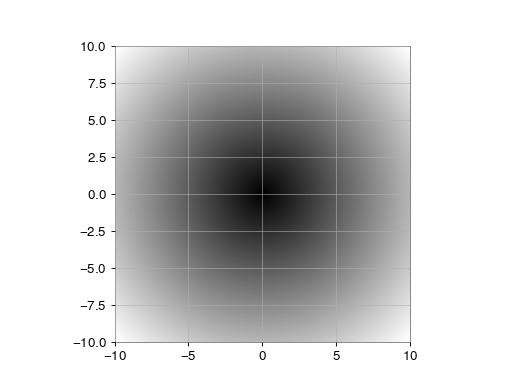
The
absfunction can be used as a shorthand fornp.absoluteon ndarrays.>>> x = np.array([-1.2, 1.2]) >>> abs(x) array([1.2, 1.2])
-
all(axis=
None, out=None, keepdims=False, *, where=True)¶ Returns True if all elements evaluate to True.
Refer to
numpy.allfor full documentation.See also
numpy.allequivalent function
-
any(axis=
None, out=None, keepdims=False, *, where=True)¶ Returns True if any of the elements of
aevaluate to True.Refer to
numpy.anyfor full documentation.See also
numpy.anyequivalent function
-
append(other, inplace=
True, pad=None, gap=None, resize=True)[source]¶ Connect another series onto the end of the current one.
- Parameters:
- other
Series another series of the same type to connect to this one
- inplace
bool, optional perform operation in-place, modifying current series, otherwise copy data and return new series, default:
TrueWarning
inplaceappend bypasses the reference check innumpy.ndarray.resize, so be carefully to only use this for arrays that haven’t been sharing their memory!- pad
float, optional value with which to pad discontiguous series, by default gaps will result in a
ValueError.- gap
str, optional action to perform if there’s a gap between the other series and this one. One of
'raise'- raise aValueError'ignore'- remove gap and join data'pad'- pad gap with zeros
If
padis given and is notNone, the default is'pad', otherwise'raise'. Ifgap='pad'is given, the default forpadis0.- resize
bool, optional resize this array to accommodate new data, otherwise shift the old data to the left (potentially falling off the start) and put the new data in at the end, default:
True.
- other
- Returns:
- series
Series a new series containing joined data sets
- series
-
argmax(axis=
None, out=None, *, keepdims=False)¶ Return indices of the maximum values along the given axis.
Refer to
numpy.argmaxfor full documentation.See also
numpy.argmaxequivalent function
-
argmin(axis=
None, out=None, *, keepdims=False)¶ Return indices of the minimum values along the given axis.
Refer to
numpy.argminfor detailed documentation.See also
numpy.argminequivalent function
-
argpartition(kth, axis=
-1, kind='introselect', order=None)¶ Returns the indices that would partition this array.
Refer to
numpy.argpartitionfor full documentation.See also
numpy.argpartitionequivalent function
-
argsort(axis=
-1, kind=None, order=None)¶ Returns the indices that would sort this array.
Refer to
numpy.argsortfor full documentation.See also
numpy.argsortequivalent function
-
asd(fftlength=
None, overlap=None, window='hann', method='median', **kwargs)[source]¶ Calculate the ASD
FrequencySeriesof thisTimeSeries- Parameters:
- fftlength
float number of seconds in single FFT, defaults to a single FFT covering the full duration
- overlap
float, optional number of seconds of overlap between FFTs, defaults to the recommended overlap for the given window (if given), or 0
- window
str,numpy.ndarray, optional window function to apply to timeseries prior to FFT, see
scipy.signal.get_window()for details on acceptable formats- method
str, optional FFT-averaging method (default:
'median'), see Notes for more details
- fftlength
- Returns:
- asd
FrequencySeries a data series containing the ASD
- asd
See also
Notes
The accepted
methodarguments are:'bartlett': a mean average of non-overlapping periodograms'median': a median average of overlapping periodograms'welch': a mean average of overlapping periodograms
-
astype(dtype, order=
'K', casting='unsafe', subok=True, copy=True)¶ Copy of the array, cast to a specified type.
- Parameters:
- dtypestr or dtype
Typecode or data-type to which the array is cast.
- order{‘C’, ‘F’, ‘A’, ‘K’}, optional
Controls the memory layout order of the result. ‘C’ means C order, ‘F’ means Fortran order, ‘A’ means ‘F’ order if all the arrays are Fortran contiguous, ‘C’ order otherwise, and ‘K’ means as close to the order the array elements appear in memory as possible. Default is ‘K’.
- casting{‘no’, ‘equiv’, ‘safe’, ‘same_kind’, ‘unsafe’}, optional
Controls what kind of data casting may occur. Defaults to ‘unsafe’ for backwards compatibility.
‘no’ means the data types should not be cast at all.
‘equiv’ means only byte-order changes are allowed.
‘safe’ means only casts which can preserve values are allowed.
‘same_kind’ means only safe casts or casts within a kind, like float64 to float32, are allowed.
‘unsafe’ means any data conversions may be done.
- subokbool, optional
If True, then sub-classes will be passed-through (default), otherwise the returned array will be forced to be a base-class array.
- copybool, optional
By default, astype always returns a newly allocated array. If this is set to false, and the
dtype,order, andsubokrequirements are satisfied, the input array is returned instead of a copy.
- Returns:
- Raises:
- ComplexWarning
When casting from complex to float or int. To avoid this, one should use
a.real.astype(t).
Examples
>>> import numpy as np
>>> x = np.array([1, 2, 2.5])
>>> x
array([1. ,  2. ,  2.5])
>>> x.astype(int) array([1, 2, 2])
-
auto_coherence(dt, fftlength=
None, overlap=None, window='hann', **kwargs)[source]¶ Calculate the frequency-coherence between this
TimeSeriesand a time-shifted copy of itself.The standard
TimeSeries.coherence()is calculated between the inputTimeSeriesand acroppedcopy of itself. Since the cropped version will be shorter, the input series will be shortened to match.- Parameters:
- dt
float duration (in seconds) of time-shift
- fftlength
float, optional number of seconds in single FFT, defaults to a single FFT covering the full duration
- overlap
float, optional number of seconds of overlap between FFTs, defaults to the recommended overlap for the given window (if given), or 0
- window
str,numpy.ndarray, optional window function to apply to timeseries prior to FFT, see
scipy.signal.get_window()for details on acceptable formats- **kwargs
any other keyword arguments accepted by
matplotlib.mlab.cohere()exceptNFFT,window, andnoverlapwhich are superceded by the above keyword arguments
- dt
- Returns:
- coherence
FrequencySeries the coherence
FrequencySeriesof thisTimeSerieswith the other
- coherence
See also
matplotlib.mlab.coherefor details of the coherence calculator
Notes
The
TimeSeries.auto_coherence()will perform best whendtis approximatelyfftlength / 2.
-
average_fft(fftlength=
None, overlap=0, window=None)[source]¶ Compute the averaged one-dimensional DFT of this
TimeSeries.This method computes a number of FFTs of duration
fftlengthandoverlap(both given in seconds), and returns the mean average. This method is analogous to the Welch average method for power spectra.- Parameters:
- fftlength
float number of seconds in single FFT, default, use whole
TimeSeries- overlap
float, optional number of seconds of overlap between FFTs, defaults to the recommended overlap for the given window (if given), or 0
- window
str,numpy.ndarray, optional window function to apply to timeseries prior to FFT, see
scipy.signal.get_window()for details on acceptable formats
- fftlength
- Returns:
- outcomplex-valued
FrequencySeries the transformed output, with populated frequencies array metadata
- outcomplex-valued
See also
TimeSeries.fftThe FFT method used.
-
bandpass(flow, fhigh, gpass=
2, gstop=30, fstop=None, type='iir', filtfilt=True, **kwargs)[source]¶ Filter this
TimeSerieswith a band-pass filter.- Parameters:
- flow
float lower corner frequency of pass band
- fhigh
float upper corner frequency of pass band
- gpass
float the maximum loss in the passband (dB).
- gstop
float the minimum attenuation in the stopband (dB).
- fstop
tupleoffloat, optional (low, high)edge-frequencies of stop band- type
str the filter type, either
'iir'or'fir'- **kwargs
other keyword arguments are passed to
gwpy.signal.filter_design.bandpass()
- flow
- Returns:
- bpseries
TimeSeries a band-passed version of the input
TimeSeries
- bpseries
See also
gwpy.signal.filter_design.bandpassfor details on the filter design
TimeSeries.filterfor details on how the filter is applied
-
byteswap(inplace=
False)¶ Swap the bytes of the array elements
Toggle between low-endian and big-endian data representation by returning a byteswapped array, optionally swapped in-place. Arrays of byte-strings are not swapped. The real and imaginary parts of a complex number are swapped individually.
- Parameters:
- inplacebool, optional
If
True, swap bytes in-place, default isFalse.
- Returns:
- outndarray
The byteswapped array. If
inplaceisTrue, this is a view to self.
Examples
>>> import numpy as np
>>> A = np.array([1, 256, 8755], dtype=np.int16)
>>> list(map(hex, A))
['0x1', '0x100', '0x2233']
>>> A.byteswap(inplace=True)
array([  256,     1, 13090], dtype=int16)
>>> list(map(hex, A))
['0x100', '0x1', '0x3322']
Arrays of byte-strings are not swapped
>>> A = np.array([b'ceg', b'fac']) >>> A.byteswap() array([b'ceg', b'fac'], dtype='|S3')A.view(A.dtype.newbyteorder()).byteswap()produces an array with the same values but different representation in memory>>> A = np.array([1, 2, 3],dtype=np.int64) >>> A.view(np.uint8) array([1, 0, 0, 0, 0, 0, 0, 0, 2, 0, 0, 0, 0, 0, 0, 0, 3, 0, 0, 0, 0, 0, 0, 0], dtype=uint8) >>> A.view(A.dtype.newbyteorder()).byteswap(inplace=True) array([1, 2, 3], dtype='>i8') >>> A.view(np.uint8) array([0, 0, 0, 0, 0, 0, 0, 1, 0, 0, 0, 0, 0, 0, 0, 2, 0, 0, 0, 0, 0, 0, 0, 3], dtype=uint8)
-
choose(choices, out=
None, mode='raise')¶ Use an index array to construct a new array from a set of choices.
Refer to
numpy.choosefor full documentation.See also
numpy.chooseequivalent function
-
clip(min=
None, max=None, out=None, **kwargs)¶ Return an array whose values are limited to
[min, max]. One of max or min must be given.Refer to
numpy.clipfor full documentation.See also
numpy.clipequivalent function
-
coherence(other, fftlength=
None, overlap=None, window='hann', **kwargs)[source]¶ Calculate the frequency-coherence between this
TimeSeriesand another.- Parameters:
- other
TimeSeries TimeSeriessignal to calculate coherence with- fftlength
float, optional number of seconds in single FFT, defaults to a single FFT covering the full duration
- overlap
float, optional number of seconds of overlap between FFTs, defaults to the recommended overlap for the given window (if given), or 0
- window
str,numpy.ndarray, optional window function to apply to timeseries prior to FFT, see
scipy.signal.get_window()for details on acceptable formats- **kwargs
any other keyword arguments accepted by
matplotlib.mlab.cohere()exceptNFFT,window, andnoverlapwhich are superceded by the above keyword arguments
- other
- Returns:
- coherence
FrequencySeries the coherence
FrequencySeriesof thisTimeSerieswith the other
- coherence
See also
scipy.signal.coherencefor details of the coherence calculator
Notes
If
selfandotherhave differenceTimeSeries.sample_ratevalues, the higher sampledTimeSerieswill be down-sampled to match the lower.
-
coherence_spectrogram(other, stride, fftlength=
None, overlap=None, window='hann', nproc=1)[source]¶ Calculate the coherence spectrogram between this
TimeSeriesand other.- Parameters:
- other
TimeSeries the second
TimeSeriesin this CSD calculation- stride
float number of seconds in single PSD (column of spectrogram)
- fftlength
float number of seconds in single FFT
- overlap
float, optional number of seconds of overlap between FFTs, defaults to the recommended overlap for the given window (if given), or 0
- window
str,numpy.ndarray, optional window function to apply to timeseries prior to FFT, see
scipy.signal.get_window()for details on acceptable formats- nproc
int number of parallel processes to use when calculating individual coherence spectra.
- other
- Returns:
- spectrogram
Spectrogram time-frequency coherence spectrogram as generated from the input time-series.
- spectrogram
-
compress(condition, axis=
None, out=None)¶ Return selected slices of this array along given axis.
Refer to
numpy.compressfor full documentation.See also
numpy.compressequivalent function
- conj()
Complex-conjugate all elements.
Refer to
numpy.conjugatefor full documentation.See also
numpy.conjugateequivalent function
- conjugate()
Return the complex conjugate, element-wise.
Refer to
numpy.conjugatefor full documentation.See also
numpy.conjugateequivalent function
-
convolve(fir, window=
'hann')[source]¶ - Convolve this
TimeSerieswith an FIR filter using the overlap-save method
- Parameters:
- fir
numpy.ndarray the time domain filter to convolve with
- window
str, optional window function to apply to boundaries, default:
'hann'seescipy.signal.get_window()for details on acceptable formats
- fir
- Returns:
- out
TimeSeries the result of the convolution
- out
See also
scipy.signal.fftconvolvefor details on the convolution scheme used here
TimeSeries.filterfor an alternative method designed for short filters
Notes
The output
TimeSeriesis the same length and has the same timestamps as the input.Due to filter settle-in, a segment half the length of
firwill be corrupted at the left and right boundaries. To prevent spectral leakage these segments will be windowed before convolving.- Convolve this
-
copy(order=
'C')[source]¶ Return a copy of the array.
- Parameters:
- order{‘C’, ‘F’, ‘A’, ‘K’}, optional
Controls the memory layout of the copy. ‘C’ means C-order, ‘F’ means F-order, ‘A’ means ‘F’ if
ais Fortran contiguous, ‘C’ otherwise. ‘K’ means match the layout ofaas closely as possible. (Note that this function andnumpy.copy()are very similar but have different default values for their order= arguments, and this function always passes sub-classes through.)
See also
numpy.copySimilar function with different default behavior
numpy.copyto
Notes
This function is the preferred method for creating an array copy. The function
numpy.copy()is similar, but it defaults to using order ‘K’, and will not pass sub-classes through by default.Examples
>>> import numpy as np
>>> x = np.array([[1,2,3],[4,5,6]], order='F')
>>> y = x.copy()>>> x.fill(0)>>> x array([[0, 0, 0], [0, 0, 0]])>>> y array([[1, 2, 3], [4, 5, 6]])>>> y.flags['C_CONTIGUOUS'] TrueFor arrays containing Python objects (e.g. dtype=object), the copy is a shallow one. The new array will contain the same object which may lead to surprises if that object can be modified (is mutable):
>>> a = np.array([1, 'm', [2, 3, 4]], dtype=object)
>>> b = a.copy()
>>> b[2][0] = 10
>>> a
array([1, 'm', list([10, 3, 4])], dtype=object)
To ensure all elements within an
objectarray are copied, usecopy.deepcopy:>>> import copy >>> a = np.array([1, 'm', [2, 3, 4]], dtype=object) >>> c = copy.deepcopy(a) >>> c[2][0] = 10 >>> c array([1, 'm', list([10, 3, 4])], dtype=object) >>> a array([1, 'm', list([2, 3, 4])], dtype=object)
-
correlate(mfilter, window=
'hann', detrend='linear', whiten=False, wduration=2, highpass=None, **asd_kw)[source]¶ Cross-correlate this
TimeSerieswith another signal- Parameters:
- mfilter
TimeSeries the time domain signal to correlate with
- window
str, optional window function to apply to timeseries prior to FFT, default:
'hann'seescipy.signal.get_window()for details on acceptable formats- detrend
str, optional type of detrending to do before FFT (see
detrendfor more details), default:'linear'- whiten
bool, optional boolean switch to enable (
True) or disable (False) data whitening, default:False- wduration
float, optional duration (in seconds) of the time-domain FIR whitening filter, only used if
whiten=True, defaults to 2 seconds- highpass
float, optional highpass corner frequency (in Hz) of the FIR whitening filter, only used if
whiten=True, default:None- **asd_kw
keyword arguments to pass to
TimeSeries.asdto generate an ASD, only used ifwhiten=True
- mfilter
- Returns:
- snr
TimeSeries the correlated signal-to-noise ratio (SNR) timeseries
- snr
See also
TimeSeries.asdfor details on the ASD calculation
TimeSeries.convolvefor details on convolution with the overlap-save method
Notes
The
windowargument is used in ASD estimation, whitening, and preventing spectral leakage in the output. It is not used to condition the matched-filter, which should be windowed before passing to this method.Due to filter settle-in, a segment half the length of
mfilterwill be corrupted at the beginning and end of the output. Seeconvolvefor more details.The input and matched-filter will be detrended, and the output will be normalised so that the SNR measures number of standard deviations from the expected mean.
-
crop(start=
None, end=None, copy=False)[source]¶ Crop this series to the given x-axis extent.
Notes
If either
startorendare outside of the originalSeriesspan, warnings will be printed and the limits will be restricted to thexspan.
-
csd(other, fftlength=
None, overlap=None, window='hann', **kwargs)[source]¶ Calculate the CSD
FrequencySeriesfor twoTimeSeries- Parameters:
- other
TimeSeries the second
TimeSeriesin this CSD calculation- fftlength
float number of seconds in single FFT, defaults to a single FFT covering the full duration
- overlap
float, optional number of seconds of overlap between FFTs, defaults to the recommended overlap for the given window (if given), or 0
- window
str,numpy.ndarray, optional window function to apply to timeseries prior to FFT, see
scipy.signal.get_window()for details on acceptable formats
- other
- Returns:
- csd
FrequencySeries a data series containing the CSD.
- csd
-
csd_spectrogram(other, stride, fftlength=
None, overlap=0, window='hann', nproc=1, **kwargs)[source]¶ - Calculate the cross spectral density spectrogram of this
TimeSerieswith ‘other’.
- Parameters:
- other
TimeSeries second time-series for cross spectral density calculation
- stride
float number of seconds in single PSD (column of spectrogram).
- fftlength
float number of seconds in single FFT.
- overlap
float, optional number of seconds of overlap between FFTs, defaults to the recommended overlap for the given window (if given), or 0
- window
str,numpy.ndarray, optional window function to apply to timeseries prior to FFT, see
scipy.signal.get_window()for details on acceptable formats- nproc
int maximum number of independent frame reading processes, default is set to single-process file reading.
- other
- Returns:
- spectrogram
Spectrogram time-frequency cross spectrogram as generated from the two input time-series.
- spectrogram
-
cumprod(axis=
None, dtype=None, out=None)¶ Return the cumulative product of the elements along the given axis.
Refer to
numpy.cumprodfor full documentation.See also
numpy.cumprodequivalent function
-
cumsum(axis=
None, dtype=None, out=None)¶ Return the cumulative sum of the elements along the given axis.
Refer to
numpy.cumsumfor full documentation.See also
numpy.cumsumequivalent function
-
decompose(bases=
[])¶ Generates a new
Quantitywith the units decomposed. Decomposed units have only irreducible units in them (seeastropy.units.UnitBase.decompose).- Parameters:
- basessequence of
UnitBase, optional The bases to decompose into. When not provided, decomposes down to any irreducible units. When provided, the decomposed result will only contain the given units. This will raises a
UnitsErrorif it’s not possible to do so.
- basessequence of
- Returns:
- newq
Quantity A new object equal to this quantity with units decomposed.
- newq
-
demodulate(f, stride=
1, exp=False, deg=True)[source]¶ Compute the average magnitude and phase of this
TimeSeriesonce per stride at a given frequency- Parameters:
- f
float frequency (Hz) at which to demodulate the signal
- stride
float, optional stride (seconds) between calculations, defaults to 1 second
- exp
bool, optional return the magnitude and phase trends as one
TimeSeriesobject representing a complex exponential, default: False- deg
bool, optional if
exp=False, calculates the phase in degrees
- f
- Returns:
- mag, phase
TimeSeries if
exp=False, returns a pair ofTimeSeriesobjects representing magnitude and phase trends withdt=stride- out
TimeSeries if
exp=True, returns a singleTimeSerieswith magnitude and phase trends represented asmag * exp(1j*phase)withdt=stride
- mag, phase
See also
TimeSeries.heterodynefor the underlying heterodyne detection method
Examples
Demodulation is useful when trying to examine steady sinusoidal signals we know to be contained within data. For instance, we can download some data from GWOSC to look at trends of the amplitude and phase of LIGO Livingston’s calibration line at 331.3 Hz:
>>> from gwpy.timeseries import TimeSeries
>>> data = TimeSeries.fetch_open_data('L1', 1131350417, 1131357617)
We can demodulate the
TimeSeriesat 331.3 Hz with a stride of one minute:>>> amp, phase = data.demodulate(331.3, stride=60)We can then plot these trends to visualize fluctuations in the amplitude of the calibration line:
>>> from gwpy.plot import Plot
>>> plot = Plot(amp)
>>> ax = plot.gca()
>>> ax.set_ylabel('Strain Amplitude at 331.3 Hz')
>>> plot.show()
(
png)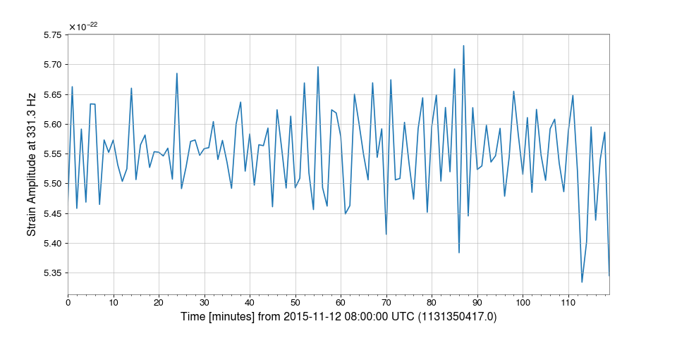
-
detrend(detrend=
'constant')[source]¶ Remove the trend from this
TimeSeriesThis method just wraps
scipy.signal.detrend()to return an object of the same type as the input.- Parameters:
- detrend
str, optional the type of detrending.
- detrend
- Returns:
- detrended
TimeSeries the detrended input series
- detrended
See also
scipy.signal.detrendfor details on the options for the
detrendargument, and how the operation is done
-
diagonal(offset=
0, axis1=0, axis2=1)¶ Return specified diagonals. In NumPy 1.9 the returned array is a read-only view instead of a copy as in previous NumPy versions. In a future version the read-only restriction will be removed.
Refer to
numpy.diagonal()for full documentation.See also
numpy.diagonalequivalent function
-
diff(n=
1, axis=-1)[source]¶ Calculate the n-th order discrete difference along given axis.
The first order difference is given by
out[n] = a[n+1] - a[n]along the given axis, higher order differences are calculated by usingdiffrecursively.- Parameters:
- nint, optional
The number of times values are differenced.
- axisint, optional
The axis along which the difference is taken, default is the last axis.
- Returns:
- diff
Series The
norder differences. The shape of the output is the same as the input, except alongaxiswhere the dimension is smaller byn.
- diff
See also
numpy.difffor documentation on the underlying method
- dumps()[source]
Returns the pickle of the array as a string. pickle.loads will convert the string back to an array.
- Parameters:
- None
-
classmethod fetch(channel, start, end, host=
None, port=None, verbose=False, connection=None, verify=False, pad=None, allow_tape=None, scaled=None, type=None, dtype=None)[source]¶ Fetch data from NDS
- Parameters:
- channel
str,Channel the data channel for which to query
- start
LIGOTimeGPS,float,str GPS start time of required data, any input parseable by
to_gpsis fine- end
LIGOTimeGPS,float,str GPS end time of required data, any input parseable by
to_gpsis fine- host
str, optional URL of NDS server to use, if blank will try any server (in a relatively sensible order) to get the data
- port
int, optional port number for NDS server query, must be given with
host- verify
bool, optional, default:False check channels exist in database before asking for data
- scaled
bool, optional apply slope and bias calibration to ADC data, for non-ADC data this option has no effect
- connection
nds2.connection, optional open NDS connection to use
- verbose
bool, optional print verbose output about NDS progress, useful for debugging; if
verboseis specified as a string, this defines the prefix for the progress meter- type
int, optional NDS2 channel type integer or string name to match
- dtype
type,numpy.dtype,str, optional NDS2 data type to match
- channel
-
classmethod fetch_open_data(ifo, start, end, sample_rate=
4096, version=None, format='hdf5', host='https://gwosc.org', verbose=False, cache=None, **kwargs)[source]¶ Fetch open-access data from the LIGO Open Science Center
- Parameters:
- ifo
str the two-character prefix of the IFO in which you are interested, e.g.
'L1'- start
LIGOTimeGPS,float,str, optional GPS start time of required data, defaults to start of data found; any input parseable by
to_gpsis fine- end
LIGOTimeGPS,float,str, optional GPS end time of required data, defaults to end of data found; any input parseable by
to_gpsis fine- sample_rate
float, optional, the sample rate of desired data; most data are stored by GWOSC at 4096 Hz, however there may be event-related data releases with a 16384 Hz rate, default:
4096- version
int, optional version of files to download, defaults to highest discovered version
- format
str, optional the data format to download and parse, default:
'h5py''hdf5''gwf'- requiresLDAStools.frameCPP
- host
str, optional HTTP host name of GWOSC server to access
- verbose
bool, optional, default:False print verbose output while fetching data
- cache
bool, optional save/read a local copy of the remote URL, default:
False; useful if the same remote data are to be accessed multiple times. SetGWPY_CACHE=1in the environment to auto-cache.- timeout
float, optional the time to wait for a response from the GWOSC server.
- **kwargs
any other keyword arguments are passed to the
TimeSeries.readmethod that parses the file that was downloaded
- ifo
Notes
StateVectordata are not available intxt.gzformat.Examples
>>> from gwpy.timeseries import (TimeSeries, StateVector)
>>> print(TimeSeries.fetch_open_data('H1', 1126259446, 1126259478))
TimeSeries([  2.17704028e-19,  2.08763900e-19,  2.39681183e-19,
            ...,   3.55365541e-20,  6.33533516e-20,
              7.58121195e-20]
           unit: Unit(dimensionless),
           t0: 1126259446.0 s,
           dt: 0.000244140625 s,
           name: Strain,
           channel: None)
>>> print(StateVector.fetch_open_data('H1', 1126259446, 1126259478))
StateVector([127,127,127,127,127,127,127,127,127,127,127,127,
             127,127,127,127,127,127,127,127,127,127,127,127,
             127,127,127,127,127,127,127,127]
            unit: Unit(dimensionless),
            t0: 1126259446.0 s,
            dt: 1.0 s,
            name: Data quality,
            channel: None,
            bits: Bits(0: data present
                       1: passes cbc CAT1 test
                       2: passes cbc CAT2 test
                       3: passes cbc CAT3 test
                       4: passes burst CAT1 test
                       5: passes burst CAT2 test
                       6: passes burst CAT3 test,
                       channel=None,
                       epoch=1126259446.0))
For the
StateVector, the naming of the bits will beformat-dependent, because they are recorded differently by GWOSC in different formats.
-
fft(nfft=
None)[source]¶ Compute the one-dimensional discrete Fourier transform of this
TimeSeries.- Parameters:
- nfft
int, optional length of the desired Fourier transform, input will be cropped or padded to match the desired length. If nfft is not given, the length of the
TimeSerieswill be used
- nfft
- Returns:
- out
FrequencySeries the normalised, complex-valued FFT
FrequencySeries.
- out
See also
numpy.fft.rfftThe FFT implementation used in this method.
Notes
This method, in constrast to the
numpy.fft.rfft()method it calls, applies the necessary normalisation such that the amplitude of the outputFrequencySeriesis correct.
-
fftgram(fftlength, overlap=
None, window='hann', **kwargs)[source]¶ Calculate the Fourier-gram of this
TimeSeries.At every
stride, a single, complex FFT is calculated.- Parameters:
- fftlength
float number of seconds in single FFT.
- overlap
float, optional number of seconds of overlap between FFTs, defaults to the recommended overlap for the given window (if given), or 0
- window
str,numpy.ndarray, optional window function to apply to timeseries prior to FFT, see
scipy.signal.get_window()for details on acceptable
- fftlength
- Returns:
- a Fourier-gram
- fill(value)
Fill the array with a scalar value.
- Parameters:
- valuescalar
All elements of
awill be assigned this value.
Examples
>>> import numpy as np
>>> a = np.array([1, 2])
>>> a.fill(0)
>>> a
array([0, 0])
>>> a = np.empty(2)
>>> a.fill(1)
>>> a
array([1.,  1.])
Fill expects a scalar value and always behaves the same as assigning to a single array element. The following is a rare example where this distinction is important:
>>> a = np.array([None, None], dtype=object)
>>> a[0] = np.array(3)
>>> a
array([array(3), None], dtype=object)
>>> a.fill(np.array(3))
>>> a
array([array(3), array(3)], dtype=object)
Where other forms of assignments will unpack the array being assigned:
>>> a[...] = np.array(3)
>>> a
array([3, 3], dtype=object)
- filter(*filt, **kwargs)[source]
Filter this
TimeSerieswith an IIR or FIR filter- Parameters:
- *filtfilter arguments
1, 2, 3, or 4 arguments defining the filter to be applied,
- filtfilt
bool, optional filter forward and backwards to preserve phase, default:
False- analog
bool, optional if
True, filter coefficients will be converted from Hz to Z-domain digital representation, default:False- inplace
bool, optional if
True, this array will be overwritten with the filtered version, default:False- **kwargs
other keyword arguments are passed to the filter method
- Returns:
- result
TimeSeries the filtered version of the input
TimeSeries
- result
- Raises:
- ValueError
if
filtarguments cannot be interpreted properly
See also
scipy.signal.sosfiltfor details on filtering with second-order sections
scipy.signal.sosfiltfiltfor details on forward-backward filtering with second-order sections
scipy.signal.lfilterfor details on filtering (without SOS)
scipy.signal.filtfiltfor details on forward-backward filtering (without SOS)
Notes
IIR filters are converted into cascading second-order sections before being applied to this
TimeSeries.FIR filters are passed directly to
scipy.signal.lfilter()orscipy.signal.filtfilt()without any conversions.Examples
We can design an arbitrarily complicated filter using
gwpy.signal.filter_design>>> from gwpy.signal import filter_design >>> bp = filter_design.bandpass(50, 250, 4096.) >>> notches = [filter_design.notch(f, 4096.) for f in (60, 120, 180)] >>> zpk = filter_design.concatenate_zpks(bp, *notches)And then can download some data from GWOSC to apply it using
TimeSeries.filter:>>> from gwpy.timeseries import TimeSeries >>> data = TimeSeries.fetch_open_data('H1', 1126259446, 1126259478) >>> filtered = data.filter(zpk, filtfilt=True)We can plot the original signal, and the filtered version, cutting off either end of the filtered data to remove filter-edge artefacts
>>> from gwpy.plot import Plot
>>> plot = Plot(data, filtered[128:-128], separate=True)
>>> plot.show()
(
png)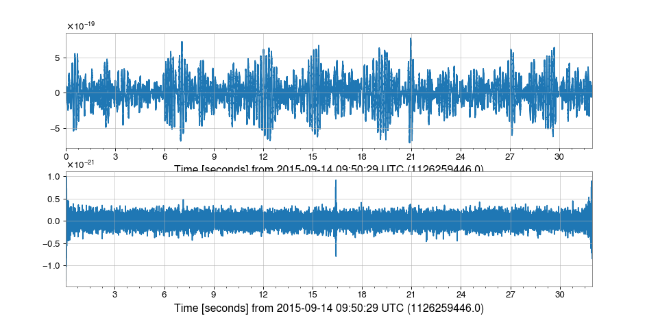
-
classmethod find(channel, start, end, frametype=
None, pad=None, scaled=None, nproc=1, verbose=False, **readargs)[source]¶ Find and read data from frames for a channel
- Parameters:
- channel
str,Channel the name of the channel to read, or a
Channelobject.- start
LIGOTimeGPS,float,str GPS start time of required data, any input parseable by
to_gpsis fine- end
LIGOTimeGPS,float,str GPS end time of required data, any input parseable by
to_gpsis fine- frametype
str, optional name of frametype in which this channel is stored, will search for containing frame types if necessary
- nproc
int, optional, default:1 number of parallel processes to use, serial process by default.
- pad
float, optional value with which to fill gaps in the source data, by default gaps will result in a
ValueError.- allow_tape
bool, optional, default:True allow reading from frame files on (slow) magnetic tape
- verbose
bool, optional print verbose output about read progress, if
verboseis specified as a string, this defines the prefix for the progress meter- **readargs
any other keyword arguments to be passed to
read()
- channel
-
find_gates(tzero=
1.0, whiten=True, threshold=50.0, cluster_window=0.5, **whiten_kwargs)[source]¶ Identify points that should be gates using a provided threshold and clustered within a provided time window.
- Parameters:
- tzero
int, optional half-width time duration (seconds) in which the timeseries is set to zero
- whiten
bool, optional if True, data will be whitened before gating points are discovered, use of this option is highly recommended
- threshold
float, optional amplitude threshold, if the data exceeds this value a gating window will be placed
- cluster_window
float, optional time duration (seconds) over which gating points will be clustered
- **whiten_kwargs
other keyword arguments that will be passed to the
TimeSeries.whitenmethod if it is being used when discovering gating points
- tzero
- Returns:
- out
SegmentList a list of segments that should be gated based on the provided parameters
- out
See also
TimeSeries.gatefor a method that applies the identified gates
-
flatten(order=
'C')[source]¶ Return a copy of the array collapsed into one dimension.
Any index information is removed as part of the flattening, and the result is returned as a
Quantityarray.- Parameters:
- order{‘C’, ‘F’, ‘A’, ‘K’}, optional
‘C’ means to flatten in row-major (C-style) order. ‘F’ means to flatten in column-major (Fortran- style) order. ‘A’ means to flatten in column-major order if
ais Fortran contiguous in memory, row-major order otherwise. ‘K’ means to flattenain the order the elements occur in memory. The default is ‘C’.
- Returns:
- y
Quantity A copy of the input array, flattened to one dimension.
- y
Examples
>>> a = Array([[1,2], [3,4]], unit='m', name='Test')
>>> a.flatten()
<Quantity [1., 2., 3., 4.] m>
-
classmethod from_lal(lalts, copy=
True)[source]¶ Generate a new TimeSeries from a LAL TimeSeries of any type.
-
classmethod from_nds2_buffer(buffer_, scaled=
None, copy=True, **metadata)[source]¶ Construct a new series from an
nds2.bufferobjectRequires:
NDS2- Parameters:
- buffer_
nds2.buffer the input NDS2-client buffer to read
- scaled
bool, optional apply slope and bias calibration to ADC data, for non-ADC data this option has no effect
- copy
bool, optional if
True, copy the contained data array to new to a new array- **metadata
any other metadata keyword arguments to pass to the
TimeSeriesconstructor
- buffer_
- Returns:
- timeseries
TimeSeries a new
TimeSeriescontaining the data from thends2.buffer, and the appropriate metadata
- timeseries
-
classmethod from_pycbc(pycbcseries, copy=
True)[source]¶ Convert a
pycbc.types.timeseries.TimeSeriesinto aTimeSeries- Parameters:
- pycbcseries
pycbc.types.timeseries.TimeSeries the input PyCBC
TimeSeriesarray- copy
bool, optional, default:True if
True, copy these data to a new array
- pycbcseries
- Returns:
- timeseries
TimeSeries a GWpy version of the input timeseries
- timeseries
-
gate(tzero=
1.0, tpad=0.5, whiten=True, threshold=50.0, cluster_window=0.5, **whiten_kwargs)[source]¶ Removes high amplitude peaks from data using inverse Planck window.
Points will be discovered automatically using a provided threshold and clustered within a provided time window.
- Parameters:
- tzero
int, optional half-width time duration (seconds) in which the timeseries is set to zero
- tpad
int, optional half-width time duration (seconds) in which the Planck window is tapered
- whiten
bool, optional if True, data will be whitened before gating points are discovered, use of this option is highly recommended
- threshold
float, optional amplitude threshold, if the data exceeds this value a gating window will be placed
- cluster_window
float, optional time duration (seconds) over which gating points will be clustered
- **whiten_kwargs
other keyword arguments that will be passed to the
TimeSeries.whitenmethod if it is being used when discovering gating points
- tzero
- Returns:
- out
TimeSeries a copy of the original
TimeSeriesthat has had gating windows applied
- out
See also
TimeSeries.maskfor the method that masks out unwanted data
TimeSeries.find_gatesfor the method that identifies gating points
TimeSeries.whitenfor the whitening filter used to identify gating points
Examples
Read data into a
TimeSeries>>> from gwpy.timeseries import TimeSeries >>> data = TimeSeries.fetch_open_data('H1', 1135148571, 1135148771)Apply gating using custom arguments
>>> gated = data.gate(tzero=1.0, tpad=1.0, threshold=10.0,
                      fftlength=4, overlap=2, method='median')
Plot the original data and the gated data, whiten both for visualization purposes
>>> overlay = data.whiten(4,2,method='median').plot(dpi=150,
                          label='Ungated', color='dodgerblue',
                          zorder=2)
>>> ax = overlay.gca()
>>> ax.plot(gated.whiten(4,2,method='median'), label='Gated',
            color='orange', zorder=3)
>>> ax.set_xlim(1135148661, 1135148681)
>>> ax.legend()
>>> overlay.show()
-
classmethod get(channel, start, end, pad=
None, scaled=None, dtype=None, verbose=False, allow_tape=None, **kwargs)[source]¶ Get data for this channel from frames or NDS
This method dynamically accesses either frames on disk, or a remote NDS2 server to find and return data for the given interval
- Parameters:
- channel
str,Channel the name of the channel to read, or a
Channelobject.- start
LIGOTimeGPS,float,str GPS start time of required data, any input parseable by
to_gpsis fine- end
LIGOTimeGPS,float,str GPS end time of required data, any input parseable by
to_gpsis fine- pad
float, optional value with which to fill gaps in the source data, by default gaps will result in a
ValueError.- scaled
bool, optional apply slope and bias calibration to ADC data, for non-ADC data this option has no effect
- nproc
int, optional, default:1 number of parallel processes to use, serial process by default.
- allow_tape
bool, optional, default:None allow the use of frames that are held on tape, default is
Noneto attempt to allow theTimeSeries.fetchmethod to intelligently select a server that doesn’t use tapes for data storage (doesn’t always work), but to eventually allow retrieving data from tape if required- verbose
bool, optional print verbose output about data access progress, if
verboseis specified as a string, this defines the prefix for the progress meter- **kwargs
other keyword arguments to pass to either
find()(for direct GWF file access) orfetch()for remote NDS2 access
- channel
See also
TimeSeries.fetchfor grabbing data from a remote NDS2 server
TimeSeries.findfor discovering and reading data from local GWF files
-
getfield(dtype, offset=
0)¶ Returns a field of the given array as a certain type.
A field is a view of the array data with a given data-type. The values in the view are determined by the given type and the offset into the current array in bytes. The offset needs to be such that the view dtype fits in the array dtype; for example an array of dtype complex128 has 16-byte elements. If taking a view with a 32-bit integer (4 bytes), the offset needs to be between 0 and 12 bytes.
- Parameters:
- dtypestr or dtype
The data type of the view. The dtype size of the view can not be larger than that of the array itself.
- offsetint
Number of bytes to skip before beginning the element view.
Examples
>>> import numpy as np
>>> x = np.diag([1.+1.j]*2)
>>> x[1, 1] = 2 + 4.j
>>> x
array([[1.+1.j,  0.+0.j],
       [0.+0.j,  2.+4.j]])
>>> x.getfield(np.float64)
array([[1.,  0.],
       [0.,  2.]])
By choosing an offset of 8 bytes we can select the complex part of the array for our view:
>>> x.getfield(np.float64, offset=8)
array([[1.,  0.],
       [0.,  4.]])
-
heterodyne(phase, stride=
1, singlesided=False)[source]¶ Compute the average magnitude and phase of this
TimeSeriesonce per stride after heterodyning with a given phase series- Parameters:
- phase
array_like an array of phase measurements (radians) with which to heterodyne the signal
- stride
float, optional stride (seconds) between calculations, defaults to 1 second
- singlesided
bool, optional Boolean switch to return single-sided output (i.e., to multiply by 2 so that the signal is distributed across positive frequencies only), default: False
- phase
- Returns:
- out
TimeSeries magnitude and phase trends, represented as
mag * exp(1j*phase)withdt=stride
- out
See also
TimeSeries.demodulatefor a method to heterodyne at a fixed frequency
Notes
This is similar to the
demodulate()method, but is more general in that it accepts a varying phase evolution, rather than a fixed frequency.Unlike
demodulate(), the complex output is double-sided by default, so is not multiplied by 2.Examples
Heterodyning can be useful in analysing quasi-monochromatic signals with a known phase evolution, such as continuous-wave signals from rapidly rotating neutron stars. These sources radiate at a frequency that slowly decreases over time, and is Doppler modulated due to the Earth’s rotational and orbital motion.
To see an example of heterodyning in action, we can simulate a signal whose phase evolution is described by the frequency and its first derivative with respect to time. We can download some O1 era LIGO-Livingston data from GWOSC, inject the simulated signal, and recover its amplitude.
>>> from gwpy.timeseries import TimeSeries
>>> data = TimeSeries.fetch_open_data('L1', 1131350417, 1131354017)
We now need to set the signal parameters, generate the expected phase evolution, and create the signal:
>>> import numpy
>>> f0 = 123.456789  # signal frequency (Hz)
>>> fdot = -9.87654321e-7  # signal frequency derivative (Hz/s)
>>> fepoch = 1131350417  # phase epoch
>>> amp = 1.5e-22  # signal amplitude
>>> phase0 = 0.4  # signal phase at the phase epoch
>>> times = data.times.value - fepoch
>>> phase = 2 * numpy.pi * (f0 * times + 0.5 * fdot * times**2)
>>> signal = TimeSeries(amp * numpy.cos(phase + phase0),
>>>                     sample_rate=data.sample_rate, t0=data.t0)
>>> data = data.inject(signal)
To recover the signal, we can bandpass the injected data around the signal frequency, then heterodyne using our phase model with a stride of 60 seconds:
>>> filtdata = data.bandpass(f0 - 0.5, f0 + 0.5)
>>> het = filtdata.heterodyne(phase, stride=60, singlesided=True)
We can then plot signal amplitude over time (cropping the first two minutes to remove the filter response):
>>> plot = het.crop(het.x0.value + 180).abs().plot()
>>> ax = plot.gca()
>>> ax.set_ylabel("Strain amplitude")
>>> plot.show()
(
png)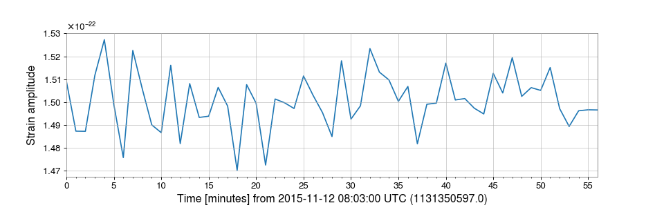
-
highpass(frequency, gpass=
2, gstop=30, fstop=None, type='iir', filtfilt=True, **kwargs)[source]¶ Filter this
TimeSerieswith a high-pass filter.- Parameters:
- frequency
float high-pass corner frequency
- gpass
float the maximum loss in the passband (dB).
- gstop
float the minimum attenuation in the stopband (dB).
- fstop
float stop-band edge frequency, defaults to
frequency * 1.5- type
str the filter type, either
'iir'or'fir'- **kwargs
other keyword arguments are passed to
gwpy.signal.filter_design.highpass()
- frequency
- Returns:
- hpseries
TimeSeries a high-passed version of the input
TimeSeries
- hpseries
See also
gwpy.signal.filter_design.highpassfor details on the filter design
TimeSeries.filterfor details on how the filter is applied
- inject(other)[source]
Add two compatible
Seriesalong their shared x-axis values.- Parameters:
- other
Series a
Serieswhose xindex intersects withself.xindex
- other
- Returns:
- out
Series the sum of
selfandotheralong their shared x-axis values
- out
- Raises:
- ValueError
if
selfandotherhave incompatible units or xindex intervals
Notes
If
other.xindexandself.xindexdo not intersect, this method will return a copy ofself. If the series have uniformly offset indices, this method will raise a warning.If
self.xindexis an array of timestamps, and ifother.xspanis not a subset ofself.xspan, thenotherwill be cropped before being adding toself.Users who wish to taper or window their
Seriesshould do so before passing it to this method. SeeTimeSeries.taper()andplanck()for more information.
-
insert(obj, values, axis=
None)¶ Insert values along the given axis before the given indices and return a new
Quantityobject.This is a thin wrapper around the
numpy.insertfunction.- Parameters:
- objint, slice or sequence of int
Object that defines the index or indices before which
valuesis inserted.- valuesarray-like
Values to insert. If the type of
valuesis different from that of quantity,valuesis converted to the matching type.valuesshould be shaped so that it can be broadcast appropriately The unit ofvaluesmust be consistent with this quantity.- axisint, optional
Axis along which to insert
values. Ifaxisis None then the quantity array is flattened before insertion.
- Returns:
- out
Quantity A copy of quantity with
valuesinserted. Note that the insertion does not occur in-place: a new quantity array is returned.
- out
Examples
>>> import astropy.units as u
>>> q = [1, 2] * u.m
>>> q.insert(0, 50 * u.cm)
<Quantity [ 0.5,  1.,  2.] m>
>>> q = [[1, 2], [3, 4]] * u.m >>> q.insert(1, [10, 20] * u.m, axis=0) <Quantity [[ 1., 2.], [ 10., 20.], [ 3., 4.]] m>>>> q.insert(1, 10 * u.m, axis=1) <Quantity [[ 1., 10., 2.], [ 3., 10., 4.]] m>
- is_compatible(other)[source]
Check whether this series and other have compatible metadata
This method tests that the
sample size, and theunitmatch.
-
is_contiguous(other, tol=
3.814697265625e-06)[source]¶ Check whether other is contiguous with self.
- Parameters:
- other
Series,numpy.ndarray another series of the same type to test for contiguity
- tol
float, optional the numerical tolerance of the test
- other
- Returns:
- 1
if
otheris contiguous with this series, i.e. would attach seamlessly onto the end
- -1
if
otheris anti-contiguous with this seires, i.e. would attach seamlessly onto the start
- 0
if
otheris completely dis-contiguous with thie series
Notes
if a raw
numpy.ndarrayis passed as other, with no metadata, then the contiguity check will always pass
- item(*args)
Copy an element of an array to a scalar Quantity and return it.
Like
item()except that it always returns aQuantity, not a Python scalar.
-
lowpass(frequency, gpass=
2, gstop=30, fstop=None, type='iir', filtfilt=True, **kwargs)[source]¶ Filter this
TimeSerieswith a Butterworth low-pass filter.- Parameters:
- frequency
float low-pass corner frequency
- gpass
float the maximum loss in the passband (dB).
- gstop
float the minimum attenuation in the stopband (dB).
- fstop
float stop-band edge frequency, defaults to
frequency * 1.5- type
str the filter type, either
'iir'or'fir'- **kwargs
other keyword arguments are passed to
gwpy.signal.filter_design.lowpass()
- frequency
- Returns:
- lpseries
TimeSeries a low-passed version of the input
TimeSeries
- lpseries
See also
gwpy.signal.filter_design.lowpassfor details on the filter design
TimeSeries.filterfor details on how the filter is applied
-
mask(deadtime=
None, flag=None, query_open_data=False, const=nan, tpad=0.5, **kwargs)[source]¶ Mask away portions of this
TimeSeriesthat fall within a given list of time segments- Parameters:
- deadtime
SegmentList, optional a list of time segments defining the deadtime (i.e., masked portions) of the output, will supersede
flagif given- flag
str, optional the name of a data-quality flag for which to query, required if
deadtimeis not given- query_open_data
bool, optional if
True, will query for publicly released data-quality segments through the Gravitational-wave Open Science Center (GWOSC), default:False- const
float, optional constant value with which to mask deadtime data, default:
nan- tpad
float, optional length of time (in seconds) over which to taper off data at mask segment boundaries, default: 0.5 seconds
- **kwargs
dict, optional additional keyword arguments to
queryorfetch_open_data, see “Notes” below
- deadtime
- Returns:
- out
TimeSeries the masked version of this
TimeSeries
- out
See also
gwpy.segments.DataQualityFlag.queryfor the method to query segments of a given data-quality flag
gwpy.segments.DataQualityFlag.fetch_open_datafor the method to query data-quality flags from the GWOSC database
gwpy.signal.window.planckfor the generic Planck-taper window
Notes
If
tpadis nonzero, the Planck-taper window is used to smoothly ramp data down to zero over a timescaletpadapproaching every segment boundary indeadtime. However, this does not apply to the left or right bounds of the originalTimeSeries.The
deadtimesegment list will always be coalesced and restricted to the limits ofself.span. In particular, when querying a data-quality flag, this means thestartandendarguments toquerywill effectively be reset and therefore need not be given.If
flagis interpreted positively, i.e. ifflagbeing active corresponds to a “good” state, then its complement inself.spanwill be used to define the deadtime for masking.
- max(axis=None, out=None, keepdims=False, initial=<no value>, where=True)
Return the maximum along a given axis.
Refer to
numpy.amaxfor full documentation.See also
numpy.amaxequivalent function
-
mean(axis=
None, dtype=None, out=None, keepdims=False, *, where=True)¶ Returns the average of the array elements along given axis.
Refer to
numpy.meanfor full documentation.See also
numpy.meanequivalent function
-
median(axis=
None, **kwargs)[source]¶ Compute the median along the specified axis.
Returns the median of the array elements.
- Parameters:
- aarray_like
Input array or object that can be converted to an array.
- axis{int, sequence of int, None}, optional
Axis or axes along which the medians are computed. The default, axis=None, will compute the median along a flattened version of the array. If a sequence of axes, the array is first flattened along the given axes, then the median is computed along the resulting flattened axis.
- outndarray, optional
Alternative output array in which to place the result. It must have the same shape and buffer length as the expected output, but the type (of the output) will be cast if necessary.
- overwrite_inputbool, optional
If True, then allow use of memory of input array
afor calculations. The input array will be modified by the call tomedian. This will save memory when you do not need to preserve the contents of the input array. Treat the input as undefined, but it will probably be fully or partially sorted. Default is False. Ifoverwrite_inputisTrueandais not already anndarray, an error will be raised.- keepdimsbool, optional
If this is set to True, the axes which are reduced are left in the result as dimensions with size one. With this option, the result will broadcast correctly against the original
arr.
- Returns:
- medianndarray
A new array holding the result. If the input contains integers or floats smaller than
float64, then the output data-type isnp.float64. Otherwise, the data-type of the output is the same as that of the input. Ifoutis specified, that array is returned instead.
See also
mean,percentile
Notes
Given a vector
Vof lengthN, the median ofVis the middle value of a sorted copy ofV,V_sorted- i e.,V_sorted[(N-1)/2], whenNis odd, and the average of the two middle values ofV_sortedwhenNis even.Examples
>>> import numpy as np
>>> a = np.array([[10, 7, 4], [3, 2, 1]])
>>> a
array([[10,  7,  4],
       [ 3,  2,  1]])
>>> np.median(a)
np.float64(3.5)
>>> np.median(a, axis=0)
array([6.5, 4.5, 2.5])
>>> np.median(a, axis=1)
array([7.,  2.])
>>> np.median(a, axis=(0, 1))
np.float64(3.5)
>>> m = np.median(a, axis=0)
>>> out = np.zeros_like(m)
>>> np.median(a, axis=0, out=m)
array([6.5,  4.5,  2.5])
>>> m
array([6.5,  4.5,  2.5])
>>> b = a.copy()
>>> np.median(b, axis=1, overwrite_input=True)
array([7.,  2.])
>>> assert not np.all(a==b)
>>> b = a.copy()
>>> np.median(b, axis=None, overwrite_input=True)
np.float64(3.5)
>>> assert not np.all(a==b)
- min(axis=None, out=None, keepdims=False, initial=<no value>, where=True)
Return the minimum along a given axis.
Refer to
numpy.aminfor full documentation.See also
numpy.aminequivalent function
- nonzero()
Return the indices of the elements that are non-zero.
Refer to
numpy.nonzerofor full documentation.See also
numpy.nonzeroequivalent function
-
notch(frequency, type=
'iir', filtfilt=True, **kwargs)[source]¶ Notch out a frequency in this
TimeSeries.- Parameters:
- frequency
float,Quantity frequency (default in Hertz) at which to apply the notch
- type
str, optional type of filter to apply, currently only ‘iir’ is supported
- **kwargs
other keyword arguments to pass to
scipy.signal.iirdesign
- frequency
- Returns:
- notched
TimeSeries a notch-filtered copy of the input
TimeSeries
- notched
See also
TimeSeries.filterfor details on the filtering method
scipy.signal.iirdesignfor details on the IIR filter design method
-
override_unit(unit, parse_strict=
'raise')[source]¶ Forcefully reset the unit of these data
Use of this method is discouraged in favour of
to(), which performs accurate conversions from one unit to another. The method should really only be used when the original unit of the array is plain wrong.
- pad(pad_width, **kwargs)[source]
Pad this series to a new size
See also
numpy.padfor details on the underlying functionality
-
partition(kth, axis=
-1, kind='introselect', order=None)¶ Partially sorts the elements in the array in such a way that the value of the element in k-th position is in the position it would be in a sorted array. In the output array, all elements smaller than the k-th element are located to the left of this element and all equal or greater are located to its right. The ordering of the elements in the two partitions on the either side of the k-th element in the output array is undefined.
- Parameters:
- kthint or sequence of ints
Element index to partition by. The kth element value will be in its final sorted position and all smaller elements will be moved before it and all equal or greater elements behind it. The order of all elements in the partitions is undefined. If provided with a sequence of kth it will partition all elements indexed by kth of them into their sorted position at once.
Deprecated since version 1.22.0: Passing booleans as index is deprecated.
- axisint, optional
Axis along which to sort. Default is -1, which means sort along the last axis.
- kind{‘introselect’}, optional
Selection algorithm. Default is ‘introselect’.
- orderstr or list of str, optional
When
ais an array with fields defined, this argument specifies which fields to compare first, second, etc. A single field can be specified as a string, and not all fields need to be specified, but unspecified fields will still be used, in the order in which they come up in the dtype, to break ties.
See also
numpy.partitionReturn a partitioned copy of an array.
argpartitionIndirect partition.
sortFull sort.
Notes
See
np.partitionfor notes on the different algorithms.Examples
>>> import numpy as np
>>> a = np.array([3, 4, 2, 1])
>>> a.partition(3)
>>> a
array([2, 1, 3, 4]) # may vary
>>> a.partition((1, 3)) >>> a array([1, 2, 3, 4])
-
plot(method=
'plot', figsize=(12, 4), xscale='auto-gps', **kwargs)[source]¶ Plot the data for this timeseries
See also
matplotlib.pyplot.figurefor documentation of keyword arguments used to create the figure
matplotlib.figure.Figure.add_subplotfor documentation of keyword arguments used to create the axes
matplotlib.axes.Axes.plotfor documentation of keyword arguments used in rendering the data
-
prepend(other, inplace=
True, pad=None, gap=None, resize=True)[source]¶ Connect another series onto the start of the current one.
- Parameters:
- other
Series another series of the same type as this one
- inplace
bool, optional perform operation in-place, modifying current series, otherwise copy data and return new series, default:
TrueWarning
inplaceprepend bypasses the reference check innumpy.ndarray.resize, so be carefully to only use this for arrays that haven’t been sharing their memory!- pad
float, optional value with which to pad discontiguous series, by default gaps will result in a
ValueError.- gap
str, optional action to perform if there’s a gap between the other series and this one. One of
'raise'- raise aValueError'ignore'- remove gap and join data'pad'- pad gap with zeros
If
padis given and is notNone, the default is'pad', otherwise'raise'.- resize
bool, optional resize this array to accommodate new data, otherwise shift the old data to the left (potentially falling off the start) and put the new data in at the end, default:
True.
- other
- Returns:
- series
TimeSeries time-series containing joined data sets
- series
-
prod(axis=
None, dtype=None, out=None, keepdims=False, initial=1, where=True)¶ Return the product of the array elements over the given axis
Refer to
numpy.prodfor full documentation.See also
numpy.prodequivalent function
-
psd(fftlength=
None, overlap=None, window='hann', method='median', **kwargs)[source]¶ Calculate the PSD
FrequencySeriesfor thisTimeSeries- Parameters:
- fftlength
float number of seconds in single FFT, defaults to a single FFT covering the full duration
- overlap
float, optional number of seconds of overlap between FFTs, defaults to the recommended overlap for the given window (if given), or 0
- window
str,numpy.ndarray, optional window function to apply to timeseries prior to FFT, see
scipy.signal.get_window()for details on acceptable formats- method
str, optional FFT-averaging method (default:
'median'), see Notes for more details- **kwargs
other keyword arguments are passed to the underlying PSD-generation method
- fftlength
- Returns:
- psd
FrequencySeries a data series containing the PSD.
- psd
Notes
The accepted
methodarguments are:'bartlett': a mean average of non-overlapping periodograms'median': a median average of overlapping periodograms'welch': a mean average of overlapping periodograms
-
put(indices, values, mode=
'raise')¶ Set
a.flat[n] = values[n]for allnin indices.Refer to
numpy.putfor full documentation.See also
numpy.putequivalent function
-
q_gram(qrange=
(4, 64), frange=(0, inf), mismatch=0.2, snrthresh=5.5, **kwargs)[source]¶ Scan a
TimeSeriesusing the multi-Q transform and return anEventTableof the most significant tiles- Parameters:
- qrange
tupleoffloat, optional (low, high)range of Qs to scan- frange
tupleoffloat, optional (low, high)range of frequencies to scan- mismatch
float, optional maximum allowed fractional mismatch between neighbouring tiles
- snrthresh
float, optional lower inclusive threshold on individual tile SNR to keep in the table
- **kwargs
other keyword arguments to be passed to
QTiling.transform(), including'epoch'and'search'
- qrange
- Returns:
- qgram
EventTable a table of time-frequency tiles on the most significant
QPlane
- qgram
See also
TimeSeries.q_transformfor a method to interpolate the raw Q-transform over a regularly gridded spectrogram
gwpy.signal.qtransformfor code and documentation on how the Q-transform is implemented
gwpy.table.EventTable.tileto render this
EventTableas a collection of polygons
Notes
Only tiles with signal energy greater than or equal to
snrthresh ** 2 / 2will be stored in the outputEventTable. The table columns are'time','duration','frequency','bandwidth', and'energy'.
-
q_transform(qrange=
(4, 64), frange=(0, inf), gps=None, search=0.5, tres='<default>', fres='<default>', logf=False, norm='median', mismatch=0.2, outseg=None, whiten=True, fduration=2, highpass=None, **asd_kw)[source]¶ Scan a
TimeSeriesusing the multi-Q transform and return an interpolated high-resolution spectrogramBy default, this method returns a high-resolution spectrogram in both time and frequency, which can result in a large memory footprint. If you know that you only need a subset of the output for, say, a figure, consider using
outsegand the other keyword arguments to restrict the size of the returned data.- Parameters:
- qrange
tupleoffloat, optional (low, high)range of Qs to scan- frange
tupleoffloat, optional (log, high)range of frequencies to scan- gps
float, optional central time of interest for determine loudest Q-plane
- search
float, optional window around
gpsin which to find peak energies, only used ifgpsis given- tres
float, optional desired time resolution (seconds) of output
Spectrogram, default isabs(outseg) / 1000.- fres
float,int,None, optional desired frequency resolution (Hertz) of output
Spectrogram, or, iflogf=True, the number of frequency samples; giveNoneto skip this step and return the original resolution, default is 0.5 Hz or 500 frequency samples- logf
bool, optional boolean switch to enable (
True) or disable (False) use of log-sampled frequencies in the outputSpectrogram, ifTruethenfresis interpreted as a number of frequency samples, default:False- norm
bool,str, optional whether to normalize the returned Q-transform output, or how, default:
True('median'), other options:False,'mean'- mismatch
float maximum allowed fractional mismatch between neighbouring tiles
- outseg
Segment, optional GPS
[start, stop)segment for outputSpectrogram, default is the full duration of the input- whiten
bool,FrequencySeries, optional boolean switch to enable (
True) or disable (False) data whitening, or an ASDFrequencySerieswith which to whiten the data- fduration
float, optional duration (in seconds) of the time-domain FIR whitening filter, only used if
whitenis notFalse, defaults to 2 seconds- highpass
float, optional highpass corner frequency (in Hz) of the FIR whitening filter, used only if
whitenis notFalse, default:None- **asd_kw
keyword arguments to pass to
TimeSeries.asdto generate an ASD to use when whitening the data
- qrange
- Returns:
- out
Spectrogram output
Spectrogramof normalised Q energy
- out
See also
TimeSeries.asdfor documentation on acceptable
**asd_kwTimeSeries.whitenfor documentation on how the whitening is done
gwpy.signal.qtransformfor code and documentation on how the Q-transform is implemented
Notes
This method will return a
Spectrogramof dtypefloat32ifnormis given, andfloat64otherwise.To optimize plot rendering with
pcolormesh, the outputSpectrogramcan be given a log-sampled frequency axis by passinglogf=Trueat runtime. Thefresargument is then the number of points on the frequency axis. Note, this is incompatible withimshow.It is also highly recommended to use the
outsegkeyword argument when only a small window around a given GPS time is of interest. This will speed up this method a little, but can greatly speed up rendering the resultingSpectrogramusingpcolormesh.If you aren’t going to use
pcolormeshin the end, don’t worry.Examples
>>> from numpy.random import normal
>>> from scipy.signal import gausspulse
>>> from gwpy.timeseries import TimeSeries
Generate a
TimeSeriescontaining Gaussian noise sampled at 4096 Hz, centred on GPS time 0, with a sine-Gaussian pulse (‘glitch’) at 500 Hz:>>> noise = TimeSeries(normal(loc=1, size=4096*4), sample_rate=4096, epoch=-2) >>> glitch = TimeSeries(gausspulse(noise.times.value, fc=500) * 4, sample_rate=4096) >>> data = noise + glitchCompute and plot the Q-transform of these data:
>>> q = data.q_transform()
>>> plot = q.plot()
>>> ax = plot.gca()
>>> ax.set_xlim(-.2, .2)
>>> ax.set_epoch(0)
>>> plot.show()
(
png)
- ravel([order])
Return a flattened array.
Refer to
numpy.ravelfor full documentation.See also
numpy.ravelequivalent function
ndarray.flata flat iterator on the array.
-
rayleigh_spectrogram(stride, fftlength=
None, overlap=0, window='hann', nproc=1, **kwargs)[source]¶ Calculate the Rayleigh statistic spectrogram of this
TimeSeries- Parameters:
- stride
float number of seconds in single PSD (column of spectrogram).
- fftlength
float number of seconds in single FFT.
- overlap
float, optional number of seconds of overlap between FFTs, passing
Nonewill choose based on the window method, default:0- window
str,numpy.ndarray, optional window function to apply to timeseries prior to FFT, see
scipy.signal.get_window()for details on acceptable formats- nproc
int, optional maximum number of independent frame reading processes, default default:
1
- stride
- Returns:
- spectrogram
Spectrogram time-frequency Rayleigh spectrogram as generated from the input time-series.
- spectrogram
See also
TimeSeries.rayleighfor details of the statistic calculation
-
rayleigh_spectrum(fftlength=
None, overlap=0, window='hann')[source]¶ Calculate the Rayleigh
FrequencySeriesfor thisTimeSeries.The Rayleigh statistic is calculated as the ratio of the standard deviation and the mean of a number of periodograms.
- Parameters:
- fftlength
float number of seconds in single FFT, defaults to a single FFT covering the full duration
- overlap
float, optional number of seconds of overlap between FFTs, passing
Nonewill choose based on the window method, default:0- window
str,numpy.ndarray, optional window function to apply to timeseries prior to FFT, see
scipy.signal.get_window()for details on acceptable formats
- fftlength
- Returns:
- psd
FrequencySeries a data series containing the PSD.
- psd
- classmethod read(source, *args, **kwargs)[source]
Read data into a
TimeSeriesArguments and keywords depend on the output format, see the online documentation for full details for each format, the parameters below are common to most formats.
- Parameters:
- source
str,list Source of data, any of the following:
- name
str,Channel the name of the channel to read, or a
Channelobject.- start
LIGOTimeGPS,float,str, optional GPS start time of required data, defaults to start of data found; any input parseable by
to_gpsis fine- end
LIGOTimeGPS,float,str, optional GPS end time of required data, defaults to end of data found; any input parseable by
to_gpsis fine- format
str, optional source format identifier. If not given, the format will be detected if possible. See below for list of acceptable formats.
- nproc
int, optional number of parallel processes to use, serial process by default.
- pad
float, optional value with which to fill gaps in the source data, by default gaps will result in a
ValueError.
- source
- Raises:
- IndexError
if
sourceis an empty list
Notes
The available built-in formats are:
Format
Read
Write
Auto-identify
csv
Yes
Yes
Yes
gwf
Yes
Yes
Yes
gwf.framecpp
Yes
Yes
No
gwf.framel
Yes
Yes
No
gwf.lalframe
Yes
Yes
No
hdf5
Yes
Yes
Yes
hdf5.gwosc
Yes
No
No
txt
Yes
Yes
Yes
wav
Yes
No
No
-
repeat(repeats, axis=
None)¶ Repeat elements of an array.
Refer to
numpy.repeatfor full documentation.See also
numpy.repeatequivalent function
-
resample(rate, window=
'hamming', ftype='fir', n=None)[source]¶ Resample this Series to a new rate
- Parameters:
- rate
float rate to which to resample this
Series- window
str,numpy.ndarray, optional window function to apply to signal in the Fourier domain, see
scipy.signal.get_window()for details on acceptable formats, only used forftype='fir'or irregular downsampling- ftype
str, optional type of filter, either ‘fir’ or ‘iir’, defaults to ‘fir’
- n
int, optional if
ftype='fir'the number of taps in the filter, otherwise the order of the Chebyshev type I IIR filter
- rate
- Returns:
- Series
a new Series with the resampling applied, and the same metadata
-
reshape(shape, /, *, order=
'C', copy=None)¶ Returns an array containing the same data with a new shape.
Refer to
numpy.reshapefor full documentation.See also
numpy.reshapeequivalent function
Notes
Unlike the free function
numpy.reshape, this method onndarrayallows the elements of the shape parameter to be passed in as separate arguments. For example,a.reshape(10, 11)is equivalent toa.reshape((10, 11)).
-
resize(new_shape, refcheck=
True)¶ Change shape and size of array in-place.
- Parameters:
- new_shapetuple of ints, or
nints Shape of resized array.
- refcheckbool, optional
If False, reference count will not be checked. Default is True.
- new_shapetuple of ints, or
- Returns:
- None
- Raises:
- ValueError
If
adoes not own its own data or references or views to it exist, and the data memory must be changed. PyPy only: will always raise if the data memory must be changed, since there is no reliable way to determine if references or views to it exist.- SystemError
If the
orderkeyword argument is specified. This behaviour is a bug in NumPy.
See also
resizeReturn a new array with the specified shape.
Notes
This reallocates space for the data area if necessary.
Only contiguous arrays (data elements consecutive in memory) can be resized.
The purpose of the reference count check is to make sure you do not use this array as a buffer for another Python object and then reallocate the memory. However, reference counts can increase in other ways so if you are sure that you have not shared the memory for this array with another Python object, then you may safely set
refcheckto False.Examples
Shrinking an array: array is flattened (in the order that the data are stored in memory), resized, and reshaped:
>>> import numpy as np>>> a = np.array([[0, 1], [2, 3]], order='C') >>> a.resize((2, 1)) >>> a array([[0], [1]])>>> a = np.array([[0, 1], [2, 3]], order='F') >>> a.resize((2, 1)) >>> a array([[0], [2]])Enlarging an array: as above, but missing entries are filled with zeros:
>>> b = np.array([[0, 1], [2, 3]])
>>> b.resize(2, 3) # new_shape parameter doesn't have to be a tuple
>>> b
array([[0, 1, 2],
       [3, 0, 0]])
Referencing an array prevents resizing…
>>> c = a
>>> a.resize((1, 1))
Traceback (most recent call last):
...
ValueError: cannot resize an array that references or is referenced ...
Unless
refcheckis False:>>> a.resize((1, 1), refcheck=False) >>> a array([[0]]) >>> c array([[0]])
-
rms(stride=
1)[source]¶ Calculate the root-mean-square value of this
TimeSeriesonce per stride.- Parameters:
- stride
float stride (seconds) between RMS calculations
- stride
- Returns:
- rms
TimeSeries a new
TimeSeriescontaining the RMS value with dt=stride
- rms
-
round(decimals=
0, out=None)¶ Return
awith each element rounded to the given number of decimals.Refer to
numpy.aroundfor full documentation.See also
numpy.aroundequivalent function
-
searchsorted(v, side=
'left', sorter=None)¶ Find indices where elements of v should be inserted in a to maintain order.
For full documentation, see
numpy.searchsortedSee also
numpy.searchsortedequivalent function
-
setfield(val, dtype, offset=
0)¶ Put a value into a specified place in a field defined by a data-type.
Place
valintoa’s field defined bydtypeand beginningoffsetbytes into the field.- Parameters:
- valobject
Value to be placed in field.
- dtypedtype object
Data-type of the field in which to place
val.- offsetint, optional
The number of bytes into the field at which to place
val.
- Returns:
- None
See also
Examples
>>> import numpy as np
>>> x = np.eye(3)
>>> x.getfield(np.float64)
array([[1.,  0.,  0.],
       [0.,  1.,  0.],
       [0.,  0.,  1.]])
>>> x.setfield(3, np.int32)
>>> x.getfield(np.int32)
array([[3, 3, 3],
       [3, 3, 3],
       [3, 3, 3]], dtype=int32)
>>> x
array([[1.0e+000, 1.5e-323, 1.5e-323],
       [1.5e-323, 1.0e+000, 1.5e-323],
       [1.5e-323, 1.5e-323, 1.0e+000]])
>>> x.setfield(np.eye(3), np.int32)
>>> x
array([[1.,  0.,  0.],
       [0.,  1.,  0.],
       [0.,  0.,  1.]])
-
setflags(write=
None, align=None, uic=None)¶ Set array flags WRITEABLE, ALIGNED, WRITEBACKIFCOPY, respectively.
These Boolean-valued flags affect how numpy interprets the memory area used by
a(see Notes below). The ALIGNED flag can only be set to True if the data is actually aligned according to the type. The WRITEBACKIFCOPY flag can never be set to True. The flag WRITEABLE can only be set to True if the array owns its own memory, or the ultimate owner of the memory exposes a writeable buffer interface, or is a string. (The exception for string is made so that unpickling can be done without copying memory.)- Parameters:
- writebool, optional
Describes whether or not
acan be written to.- alignbool, optional
Describes whether or not
ais aligned properly for its type.- uicbool, optional
Describes whether or not
ais a copy of another “base” array.
Notes
Array flags provide information about how the memory area used for the array is to be interpreted. There are 7 Boolean flags in use, only three of which can be changed by the user: WRITEBACKIFCOPY, WRITEABLE, and ALIGNED.
WRITEABLE (W) the data area can be written to;
ALIGNED (A) the data and strides are aligned appropriately for the hardware (as determined by the compiler);
WRITEBACKIFCOPY (X) this array is a copy of some other array (referenced by .base). When the C-API function PyArray_ResolveWritebackIfCopy is called, the base array will be updated with the contents of this array.
All flags can be accessed using the single (upper case) letter as well as the full name.
Examples
>>> import numpy as np
>>> y = np.array([[3, 1, 7],
...               [2, 0, 0],
...               [8, 5, 9]])
>>> y
array([[3, 1, 7],
       [2, 0, 0],
       [8, 5, 9]])
>>> y.flags
  C_CONTIGUOUS : True
  F_CONTIGUOUS : False
  OWNDATA : True
  WRITEABLE : True
  ALIGNED : True
  WRITEBACKIFCOPY : False
>>> y.setflags(write=0, align=0)
>>> y.flags
  C_CONTIGUOUS : True
  F_CONTIGUOUS : False
  OWNDATA : True
  WRITEABLE : False
  ALIGNED : False
  WRITEBACKIFCOPY : False
>>> y.setflags(uic=1)
Traceback (most recent call last):
  File "<stdin>", line 1, in <module>
ValueError: cannot set WRITEBACKIFCOPY flag to True
- shift(delta)[source]
Shift this
Seriesforward on the X-axis bydeltaThis modifies the series in-place.
- Parameters:
Examples
>>> from gwpy.types import Series
>>> a = Series([1, 2, 3, 4, 5], x0=0, dx=1, xunit='m')
>>> print(a.x0)
0.0 m
>>> a.shift(5)
>>> print(a.x0)
5.0 m
>>> a.shift('-1 km')
-995.0 m
-
sort(axis=
-1, kind=None, order=None)¶ Sort an array in-place. Refer to
numpy.sortfor full documentation.- Parameters:
- axisint, optional
Axis along which to sort. Default is -1, which means sort along the last axis.
- kind{‘quicksort’, ‘mergesort’, ‘heapsort’, ‘stable’}, optional
Sorting algorithm. The default is ‘quicksort’. Note that both ‘stable’ and ‘mergesort’ use timsort under the covers and, in general, the actual implementation will vary with datatype. The ‘mergesort’ option is retained for backwards compatibility.
- orderstr or list of str, optional
When
ais an array with fields defined, this argument specifies which fields to compare first, second, etc. A single field can be specified as a string, and not all fields need be specified, but unspecified fields will still be used, in the order in which they come up in the dtype, to break ties.
See also
numpy.sortReturn a sorted copy of an array.
numpy.argsortIndirect sort.
numpy.lexsortIndirect stable sort on multiple keys.
numpy.searchsortedFind elements in sorted array.
numpy.partitionPartial sort.
Notes
See
numpy.sortfor notes on the different sorting algorithms.Examples
>>> import numpy as np
>>> a = np.array([[1,4], [3,1]])
>>> a.sort(axis=1)
>>> a
array([[1, 4],
       [1, 3]])
>>> a.sort(axis=0)
>>> a
array([[1, 3],
       [1, 4]])
Use the
orderkeyword to specify a field to use when sorting a structured array:>>> a = np.array([('a', 2), ('c', 1)], dtype=[('x', 'S1'), ('y', int)]) >>> a.sort(order='y') >>> a array([(b'c', 1), (b'a', 2)], dtype=[('x', 'S1'), ('y', '<i8')])
-
spectral_variance(stride, fftlength=
None, overlap=None, method='median', window='hann', nproc=1, filter=None, bins=None, low=None, high=None, nbins=500, log=False, norm=False, density=False)[source]¶ Calculate the
SpectralVarianceof thisTimeSeries.- Parameters:
- stride
float number of seconds in single PSD (column of spectrogram)
- fftlength
float number of seconds in single FFT
- method
str, optional FFT-averaging method (default:
'median'), see Notes for more details- overlap
float, optional number of seconds of overlap between FFTs, defaults to the recommended overlap for the given window (if given), or 0
- window
str,numpy.ndarray, optional window function to apply to timeseries prior to FFT, see
scipy.signal.get_window()for details on acceptable formats- nproc
int maximum number of independent frame reading processes, default is set to single-process file reading.
- bins
numpy.ndarray, optional, defaultNone array of histogram bin edges, including the rightmost edge
- low
float, optional left edge of lowest amplitude bin, only read if
binsis not given- high
float, optional right edge of highest amplitude bin, only read if
binsis not given- nbins
int, optional number of bins to generate, only read if
binsis not given- log
bool, optional calculate amplitude bins over a logarithmic scale, only read if
binsis not given- norm
bool, optional normalise bin counts to a unit sum
- density
bool, optional normalise bin counts to a unit integral
- stride
- Returns:
- specvar
SpectralVariance 2D-array of spectral frequency-amplitude counts
- specvar
See also
numpy.histogramfor details on specifying bins and weights
Notes
The accepted
methodarguments are:'bartlett': a mean average of non-overlapping periodograms'median': a median average of overlapping periodograms'welch': a mean average of overlapping periodograms
-
spectrogram(stride, fftlength=
None, overlap=None, window='hann', method='median', nproc=1, **kwargs)[source]¶ Calculate the average power spectrogram of this
TimeSeriesusing the specified average spectrum method.Each time-bin of the output
Spectrogramis calculated by taking a chunk of theTimeSeriesin the segment[t - overlap/2., t + stride + overlap/2.)and calculating thepsd()of those data.As a result, each time-bin is calculated using
stride + overlapseconds of data.- Parameters:
- stride
float number of seconds in single PSD (column of spectrogram).
- fftlength
float number of seconds in single FFT.
- overlap
float, optional number of seconds of overlap between FFTs, defaults to the recommended overlap for the given window (if given), or 0
- window
str,numpy.ndarray, optional window function to apply to timeseries prior to FFT, see
scipy.signal.get_window()for details on acceptable formats- method
str, optional FFT-averaging method (default:
'median'), see Notes for more details- nproc
int number of CPUs to use in parallel processing of FFTs
- stride
- Returns:
- spectrogram
Spectrogram time-frequency power spectrogram as generated from the input time-series.
- spectrogram
Notes
The accepted
methodarguments are:'bartlett': a mean average of non-overlapping periodograms'median': a median average of overlapping periodograms'welch': a mean average of overlapping periodograms
-
spectrogram2(fftlength, overlap=
None, window='hann', **kwargs)[source]¶ Calculate the non-averaged power
Spectrogramof thisTimeSeries- Parameters:
- fftlength
float number of seconds in single FFT.
- overlap
float, optional number of seconds of overlap between FFTs, defaults to the recommended overlap for the given window (if given), or 0
- window
str,numpy.ndarray, optional window function to apply to timeseries prior to FFT, see
scipy.signal.get_window()for details on acceptable formats- scaling[ ‘density’ | ‘spectrum’ ], optional
selects between computing the power spectral density (‘density’) where the
Spectrogramhas units of V**2/Hz if the input is measured in V and computing the power spectrum (‘spectrum’) where theSpectrogramhas units of V**2 if the input is measured in V. Defaults to ‘density’.- **kwargs
other parameters to be passed to
scipy.signal.periodogramfor each column of theSpectrogram
- fftlength
- Returns:
- spectrogram:
Spectrogram a power
Spectrogramwith1/fftlengthfrequency resolution and (fftlength - overlap) time resolution.
- spectrogram:
See also
scipy.signal.periodogramfor documentation on the Fourier methods used in this calculation
Notes
This method calculates overlapping periodograms for all possible chunks of data entirely containing within the span of the input
TimeSeries, then normalises the power in overlapping chunks using a triangular window centred on that chunk which most overlaps the givenSpectrogramtime sample.
-
squeeze(axis=
None)¶ Remove axes of length one from
a.Refer to
numpy.squeezefor full documentation.See also
numpy.squeezeequivalent function
-
std(axis=
None, dtype=None, out=None, ddof=0, keepdims=False, *, where=True)¶ Returns the standard deviation of the array elements along given axis.
Refer to
numpy.stdfor full documentation.See also
numpy.stdequivalent function
-
sum(axis=
None, dtype=None, out=None, keepdims=False, initial=0, where=True)¶ Return the sum of the array elements over the given axis.
Refer to
numpy.sumfor full documentation.See also
numpy.sumequivalent function
- swapaxes(axis1, axis2)
Return a view of the array with
axis1andaxis2interchanged.Refer to
numpy.swapaxesfor full documentation.See also
numpy.swapaxesequivalent function
-
take(indices, axis=
None, out=None, mode='raise')¶ Return an array formed from the elements of
aat the given indices.Refer to
numpy.takefor full documentation.See also
numpy.takeequivalent function
-
taper(side=
'leftright', duration=None, nsamples=None)[source]¶ Taper the ends of this
TimeSeriessmoothly to zero.- Parameters:
- side
str, optional the side of the
TimeSeriesto taper, must be one of'left','right', or'leftright'- duration
float, optional the duration of time to taper, will override
nsamplesif both are provided as arguments- nsamples
int, optional the number of samples to taper, will be overridden by
durationif both are provided as arguments
- side
- Returns:
- out
TimeSeries a copy of
selftapered at one or both ends
- out
- Raises:
- ValueError
if
sideis not one of('left', 'right', 'leftright')
Notes
The
TimeSeries.taper()automatically tapers from the second stationary point (local maximum or minimum) on the specified side of the input. However, the method will never taper more than half the full width of theTimeSeries, and will fail if there are no stationary points.See
planck()for the generic Planck taper window, and seescipy.signal.get_window()for other common window formats.Examples
To see the effect of the Planck-taper window, we can taper a sinusoidal
TimeSeriesat both ends:>>> import numpy >>> from gwpy.timeseries import TimeSeries >>> t = numpy.linspace(0, 1, 2048) >>> series = TimeSeries(numpy.cos(10.5*numpy.pi*t), times=t) >>> tapered = series.taper()We can plot it to see how the ends now vary smoothly from 0 to 1:
>>> from gwpy.plot import Plot
>>> plot = Plot(series, tapered, separate=True, sharex=True)
>>> plot.show()
(
png)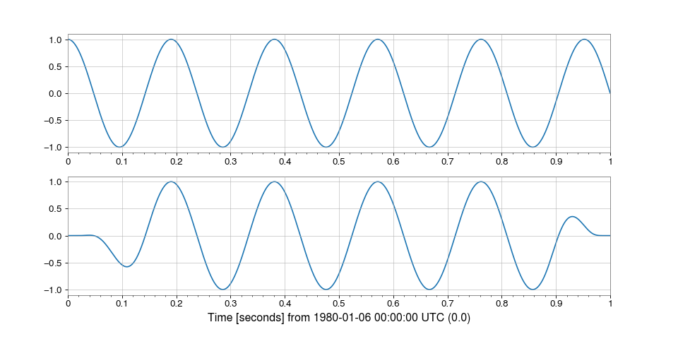
-
to(unit, equivalencies=
[], copy=True)¶ Return a new
Quantityobject with the specified unit.- Parameters:
- unitunit-like
An object that represents the unit to convert to. Must be an
UnitBaseobject or a string parseable by theunitspackage.- equivalencieslist of tuple
A list of equivalence pairs to try if the units are not directly convertible. See Equivalencies. If not provided or
[], class default equivalencies will be used (none forQuantity, but may be set for subclasses) IfNone, no equivalencies will be applied at all, not even any set globally or within a context.- copybool, optional
If
True(default), then the value is copied. Otherwise, a copy will only be made if necessary.
See also
to_valueget the numerical value in a given unit.
- to_device()
- to_lal()[source]
Convert this
TimeSeriesinto a LAL TimeSeries.Note
This operation always copies data to new memory.
-
to_pycbc(copy=
True)[source]¶ Convert this
TimeSeriesinto a PyCBCTimeSeries- Parameters:
- Returns:
- timeseries
TimeSeries a PyCBC representation of this
TimeSeries
- timeseries
-
to_string(unit=
None, precision=None, format=None, subfmt=None, *, formatter=None)¶ Generate a string representation of the quantity and its unit.
The behavior of this function can be altered via the
numpy.set_printoptionsfunction and its various keywords. The exception to this is thethresholdkeyword, which is controlled via the[units.quantity]configuration itemlatex_array_threshold. This is treated separately because the numpy default of 1000 is too big for most browsers to handle.- Parameters:
- unitunit-like, optional
Specifies the unit. If not provided, the unit used to initialize the quantity will be used.
- precisionnumber, optional
The level of decimal precision. If
None, or not provided, it will be determined from NumPy print options.- formatstr, optional
The format of the result. If not provided, an unadorned string is returned. Supported values are:
‘latex’: Return a LaTeX-formatted string
‘latex_inline’: Return a LaTeX-formatted string that uses negative exponents instead of fractions
- formatterstr, callable, dict, optional
The formatter to use for the value. If a string, it should be a valid format specifier using Python’s mini-language. If a callable, it will be treated as the default formatter for all values and will overwrite default Latex formatting for exponential notation and complex numbers. If a dict, it should map a specific type to a callable to be directly passed into
numpy.array2string. If not provided, the default formatter will be used.- subfmtstr, optional
Subformat of the result. For the moment, only used for
format='latex'andformat='latex_inline'. Supported values are:‘inline’: Use
$ ... $as delimiters.‘display’: Use
$\displaystyle ... $as delimiters.
- Returns:
- str
A string with the contents of this Quantity
-
to_value(unit=
None, equivalencies=[])¶ The numerical value, possibly in a different unit.
- Parameters:
- unitunit-like, optional
The unit in which the value should be given. If not given or
None, use the current unit.- equivalencieslist of tuple, optional
A list of equivalence pairs to try if the units are not directly convertible (see Equivalencies). If not provided or
[], class default equivalencies will be used (none forQuantity, but may be set for subclasses). IfNone, no equivalencies will be applied at all, not even any set globally or within a context.
- Returns:
- valuendarray or scalar
The value in the units specified. For arrays, this will be a view of the data if no unit conversion was necessary.
See also
toGet a new instance in a different unit.
- tolist()
Return the array as an
a.ndim-levels deep nested list of Python scalars.Return a copy of the array data as a (nested) Python list. Data items are converted to the nearest compatible builtin Python type, via the
itemfunction.If
a.ndimis 0, then since the depth of the nested list is 0, it will not be a list at all, but a simple Python scalar.- Parameters:
- none
- Returns:
- yobject, or list of object, or list of list of object, or …
The possibly nested list of array elements.
Notes
The array may be recreated via
a = np.array(a.tolist()), although this may sometimes lose precision.Examples
For a 1D array,
a.tolist()is almost the same aslist(a), except thattolistchanges numpy scalars to Python scalars:>>> import numpy as np >>> a = np.uint32([1, 2]) >>> a_list = list(a) >>> a_list [np.uint32(1), np.uint32(2)] >>> type(a_list[0]) <class 'numpy.uint32'> >>> a_tolist = a.tolist() >>> a_tolist [1, 2] >>> type(a_tolist[0]) <class 'int'>Additionally, for a 2D array,
tolistapplies recursively:>>> a = np.array([[1, 2], [3, 4]]) >>> list(a) [array([1, 2]), array([3, 4])] >>> a.tolist() [[1, 2], [3, 4]]The base case for this recursion is a 0D array:
>>> a = np.array(1)
>>> list(a)
Traceback (most recent call last):
  ...
TypeError: iteration over a 0-d array
>>> a.tolist()
1
-
tostring(order=
'C')[source]¶ Construct Python bytes containing the raw data bytes in the array.
Constructs Python bytes showing a copy of the raw contents of data memory. The bytes object is produced in C-order by default. This behavior is controlled by the
orderparameter.- Parameters:
- order{‘C’, ‘F’, ‘A’}, optional
Controls the memory layout of the bytes object. ‘C’ means C-order, ‘F’ means F-order, ‘A’ (short for Any) means ‘F’ if
ais Fortran contiguous, ‘C’ otherwise. Default is ‘C’.
- Returns:
- sbytes
Python bytes exhibiting a copy of
a’s raw data.
See also
frombufferInverse of this operation, construct a 1-dimensional array from Python bytes.
Examples
>>> import numpy as np
>>> x = np.array([[0, 1], [2, 3]], dtype='<u2')
>>> x.tobytes()
b'\x00\x00\x01\x00\x02\x00\x03\x00'
>>> x.tobytes('C') == x.tobytes()
True
>>> x.tobytes('F')
b'\x00\x00\x02\x00\x01\x00\x03\x00'
-
trace(offset=
0, axis1=0, axis2=1, dtype=None, out=None)¶ Return the sum along diagonals of the array.
Refer to
numpy.tracefor full documentation.See also
numpy.traceequivalent function
-
transfer_function(other, fftlength=
None, overlap=None, window='hann', average='mean', **kwargs)[source]¶ Calculate the transfer function between this
TimeSeriesand another.This
TimeSeriesis the ‘A-channel’, serving as the reference (denominator) while the other time series is the test (numerator)- Parameters:
- other
TimeSeries TimeSeriessignal to calculate the transfer function with- fftlength
float, optional number of seconds in single FFT, defaults to a single FFT covering the full duration
- overlap
float, optional number of seconds of overlap between FFTs, defaults to the recommended overlap for the given window (if given), or 0
- window
str,numpy.ndarray, optional window function to apply to timeseries prior to FFT, see
scipy.signal.get_window()for details on acceptable formats- average
str, optional FFT-averaging method (default:
'mean') passed to underlying csd() and psd() methods- **kwargs
any other keyword arguments accepted by
TimeSeries.csd()orTimeSeries.psd()
- other
- Returns:
- transfer_function
FrequencySeries the transfer function
FrequencySeriesof thisTimeSerieswith the other
- transfer_function
Notes
If
selfandotherhave differenceTimeSeries.sample_ratevalues, the higher sampledTimeSerieswill be down-sampled to match the lower.
- transpose(*axes)
Returns a view of the array with axes transposed.
Refer to
numpy.transposefor full documentation.- Parameters:
- axesNone, tuple of ints, or
nints None or no argument: reverses the order of the axes.
tuple of ints:
iin thej-th place in the tuple means that the array’si-th axis becomes the transposed array’sj-th axis.nints: same as an n-tuple of the same ints (this form is intended simply as a “convenience” alternative to the tuple form).
- axesNone, tuple of ints, or
- Returns:
- pndarray
View of the array with its axes suitably permuted.
See also
transposeEquivalent function.
ndarray.TArray property returning the array transposed.
ndarray.reshapeGive a new shape to an array without changing its data.
Examples
>>> import numpy as np
>>> a = np.array([[1, 2], [3, 4]])
>>> a
array([[1, 2],
       [3, 4]])
>>> a.transpose()
array([[1, 3],
       [2, 4]])
>>> a.transpose((1, 0))
array([[1, 3],
       [2, 4]])
>>> a.transpose(1, 0)
array([[1, 3],
       [2, 4]])
>>> a = np.array([1, 2, 3, 4]) >>> a array([1, 2, 3, 4]) >>> a.transpose() array([1, 2, 3, 4])
-
update(other, inplace=
True)[source]¶ Update this series by appending new data from an other and dropping the same amount of data off the start.
This is a convenience method that just calls
appendwithresize=False.
-
var(axis=
None, dtype=None, out=None, ddof=0, keepdims=False, *, where=True)¶ Returns the variance of the array elements, along given axis.
Refer to
numpy.varfor full documentation.See also
numpy.varequivalent function
- view([dtype][, type])
New view of array with the same data.
Note
Passing None for
dtypeis different from omitting the parameter, since the former invokesdtype(None)which is an alias fordtype('float64').- Parameters:
- dtypedata-type or ndarray sub-class, optional
Data-type descriptor of the returned view, e.g., float32 or int16. Omitting it results in the view having the same data-type as
a. This argument can also be specified as an ndarray sub-class, which then specifies the type of the returned object (this is equivalent to setting thetypeparameter).- typePython type, optional
Type of the returned view, e.g., ndarray or matrix. Again, omission of the parameter results in type preservation.
Notes
a.view()is used two different ways:a.view(some_dtype)ora.view(dtype=some_dtype)constructs a view of the array’s memory with a different data-type. This can cause a reinterpretation of the bytes of memory.a.view(ndarray_subclass)ora.view(type=ndarray_subclass)just returns an instance ofndarray_subclassthat looks at the same array (same shape, dtype, etc.) This does not cause a reinterpretation of the memory.For
a.view(some_dtype), ifsome_dtypehas a different number of bytes per entry than the previous dtype (for example, converting a regular array to a structured array), then the last axis ofamust be contiguous. This axis will be resized in the result.Changed in version 1.23.0: Only the last axis needs to be contiguous. Previously, the entire array had to be C-contiguous.
Examples
>>> import numpy as np
>>> x = np.array([(-1, 2)], dtype=[('a', np.int8), ('b', np.int8)])
Viewing array data using a different type and dtype:
>>> nonneg = np.dtype([("a", np.uint8), ("b", np.uint8)])
>>> y = x.view(dtype=nonneg, type=np.recarray)
>>> x["a"]
array([-1], dtype=int8)
>>> y.a
array([255], dtype=uint8)
Creating a view on a structured array so it can be used in calculations
>>> x = np.array([(1, 2),(3,4)], dtype=[('a', np.int8), ('b', np.int8)])
>>> xv = x.view(dtype=np.int8).reshape(-1,2)
>>> xv
array([[1, 2],
       [3, 4]], dtype=int8)
>>> xv.mean(0)
array([2.,  3.])
Making changes to the view changes the underlying array
>>> xv[0,1] = 20
>>> x
array([(1, 20), (3,  4)], dtype=[('a', 'i1'), ('b', 'i1')])
Using a view to convert an array to a recarray:
>>> z = x.view(np.recarray)
>>> z.a
array([1, 3], dtype=int8)
Views share data:
>>> x[0] = (9, 10)
>>> z[0]
np.record((9, 10), dtype=[('a', 'i1'), ('b', 'i1')])
Views that change the dtype size (bytes per entry) should normally be avoided on arrays defined by slices, transposes, fortran-ordering, etc.:
>>> x = np.array([[1, 2, 3], [4, 5, 6]], dtype=np.int16)
>>> y = x[:, ::2]
>>> y
array([[1, 3],
       [4, 6]], dtype=int16)
>>> y.view(dtype=[('width', np.int16), ('length', np.int16)])
Traceback (most recent call last):
    ...
ValueError: To change to a dtype of a different size, the last axis must be contiguous
>>> z = y.copy()
>>> z.view(dtype=[('width', np.int16), ('length', np.int16)])
array([[(1, 3)],
       [(4, 6)]], dtype=[('width', '<i2'), ('length', '<i2')])
However, views that change dtype are totally fine for arrays with a contiguous last axis, even if the rest of the axes are not C-contiguous:
>>> x = np.arange(2 * 3 * 4, dtype=np.int8).reshape(2, 3, 4)
>>> x.transpose(1, 0, 2).view(np.int16)
array([[[ 256,  770],
        [3340, 3854]],

       [[1284, 1798],
        [4368, 4882]],

       [[2312, 2826],
        [5396, 5910]]], dtype=int16)
-
whiten(fftlength=
None, overlap=0, method='median', window='hann', detrend='constant', asd=None, fduration=2, highpass=None, **kwargs)[source]¶ Whiten this
TimeSeriesusing inverse spectrum truncation- Parameters:
- fftlength
float, optional FFT integration length (in seconds) for ASD estimation, default: choose based on sample rate
- overlap
float, optional number of seconds of overlap between FFTs, defaults to the recommended overlap for the given window (if given), or 0
- method
str, optional FFT-averaging method (default:
'median')- window
str,numpy.ndarray, optional window function to apply to timeseries prior to FFT, default:
'hann'seescipy.signal.get_window()for details on acceptable formats- detrend
str, optional type of detrending to do before FFT (see
detrendfor more details), default:'constant'- asd
FrequencySeries, optional the amplitude spectral density using which to whiten the data, overrides other ASD arguments, default:
None- fduration
float, optional duration (in seconds) of the time-domain FIR whitening filter, must be no longer than
fftlength, default: 2 seconds- highpass
float, optional highpass corner frequency (in Hz) of the FIR whitening filter, default:
None- **kwargs
other keyword arguments are passed to the
TimeSeries.asdmethod to estimate the amplitude spectral densityFrequencySeriesof thisTimeSeries
- fftlength
- Returns:
- out
TimeSeries a whitened version of the input data with zero mean and unit variance
- out
See also
TimeSeries.asdfor details on the ASD calculation
TimeSeries.convolvefor details on convolution with the overlap-save method
gwpy.signal.filter_design.fir_from_transferfor FIR filter design through spectrum truncation
Notes
The accepted
methodarguments are:'bartlett': a mean average of non-overlapping periodograms'median': a median average of overlapping periodograms'welch': a mean average of overlapping periodograms
The
windowargument is used in ASD estimation, FIR filter design, and in preventing spectral leakage in the output.Due to filter settle-in, a segment of length
0.5*fdurationwill be corrupted at the beginning and end of the output. Seeconvolvefor more details.The input is detrended and the output normalised such that, if the input is stationary and Gaussian, then the output will have zero mean and unit variance.
For more on inverse spectrum truncation, see arXiv:gr-qc/0509116.
- write(target, *args, **kwargs)[source]
Write this
TimeSeriesto a file- Parameters:
Notes
The available built-in formats are:
Format
Read
Write
Auto-identify
csv
Yes
Yes
Yes
gwf
Yes
Yes
Yes
gwf.framecpp
Yes
Yes
No
gwf.framel
Yes
Yes
No
gwf.lalframe
Yes
Yes
No
hdf5
Yes
Yes
Yes
txt
Yes
Yes
Yes
wav
Yes
Yes
No
- zip()[source]
Zip the
xindexandvaluearrays of thisSeries- Returns:
- stacked2-d
numpy.ndarray The array formed by stacking the the
xindexandvalueof this series
- stacked2-d
Examples
>>> a = Series([0, 2, 4, 6, 8], xindex=[-5, -4, -3, -2, -1])
>>> a.zip()
array([[-5.,  0.],
       [-4.,  2.],
       [-3.,  4.],
       [-2.,  6.],
       [-1.,  8.]])
-
zpk(zeros, poles, gain, analog=
True, **kwargs)[source]¶ Filter this
TimeSeriesby applying a zero-pole-gain filter- Parameters:
- Returns:
- timeseries
TimeSeries the filtered version of the input data
- timeseries
See also
TimeSeries.filterfor details on how a digital ZPK-format filter is applied
Examples
To apply a zpk filter with file poles at 100 Hz, and five zeros at 1 Hz (giving an overall DC gain of 1e-10):
>>> data2 = data.zpk([100]*5, [1]*5, 1e-10)
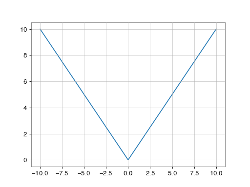
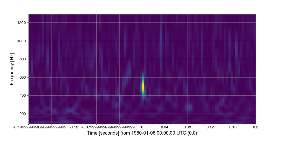