Signal processing¶

In a wide-array of applications, the original data recorded from a digital system must be manipulated in order to extract the greatest amount of information. GWpy provides a suite of functions to simplify and extend the excellent digital signal processing suite in scipy.signal.

Spectral density estimation¶

Spectral density estimation is a common way of investigating the frequency-domain content of a time-domain signal. GWpy provides wrappers of power spectral density (PSD) estimation methods from scipy.signal to simplify calculating a FrequencySeries from a TimeSeries.

The gwpy.signal.spectral sub-package provides the following PSD estimation averaging methods:

• 'bartlett' - mean average of non-overlapping periodograms

• 'median' - median average of overlapping periodograms

• 'welch' - mean average of overlapping periodograms

Each of these can be specified by passing the function name as the method keyword argument to any of the relevant TimeSeries instance methods:

e.g, TimeSeries.psd():

>>> ts = TimeSeries(...)
>>> psd = ts.psd(..., method='median', ...)

See scipy.signal.welch() for more detailed documentation on the PSD estimation method used.

Time-domain filtering¶

The TimeSeries object comes with a number of instance methods that should make filtering data trivial for a number of common use cases. Available methods include:

Each of the above methods eventually calls out to TimeSeries.filter() to apply a digital linear filter, normally via cascaded second-order-sections (requires scipy >= 0.16).

For a worked example of how to filter LIGO data to discover a gravitational-wave signal, see the example Filtering a TimeSeries to detect gravitational waves.

Frequency-domain filtering¶

Additionally, the TimeSeries object includes a number of instance methods to generate frequency-domain information for some data. Available methods include:

For a worked example of how to load data and calculate the Amplitude Spectral Density FrequencySeries, see the example Calculating and plotting a FrequencySeries.

Filter design¶

The gwpy.signal provides a number of filter design methods which, when combined with the BodePlot visualisation, can be used to create a number of common filters:

Each of these will return filter coefficients that can be passed directly into zpk (default for analogue filters) or filter (default for digital filters).

For a worked example of how to filter LIGO data to discover a gravitational-wave signal, see the example Filtering a TimeSeries to detect gravitational waves.

Cross-channel correlations:

For a worked example of how to compare channels like this, see the example Calculating the coherence between two channels.

Reference/API¶

filter_design.bandpass(fhigh, sample_rate, fstop=None, gpass=2, gstop=30, type='iir', **kwargs)[source]¶

Design a band-pass filter for the given cutoff frequencies

Parameters:¶

flowfloat

lower corner frequency of pass band

fhighfloat

upper corner frequency of pass band

sample_ratefloat

sampling rate of target data

fstoptuple of float, optional

(low, high) edge-frequencies of stop band

gpassfloat, optional, default: 2

the maximum loss in the passband (dB)

gstopfloat, optional, default: 30

the minimum attenuation in the stopband (dB)

typestr, optional, default: 'iir'

the filter type, either 'iir' or 'fir'

**kwargs

other keyword arguments are passed directly to iirdesign() or firwin()

Returns:¶

filter

the formatted filter. the output format for an IIR filter depends on the input arguments, default is a tuple of (zeros, poles, gain)

Notes

By default a digital filter is returned, meaning the zeros and poles are given in the Z-domain in units of radians/sample.

Examples

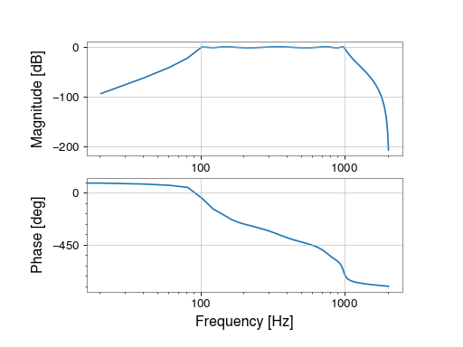
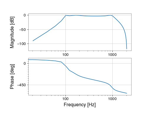
To create a band-pass filter for 100-1000 Hz for 4096 Hz-sampled data:

>>> from gwpy.signal.filter_design import bandpass
>>> bp = bandpass(100, 1000, 4096)

To view the filter, you can use the BodePlot:

>>> from gwpy.plot import BodePlot
>>> plot = BodePlot(bp, sample_rate=4096)
>>> plot.show()

(png)

filter_design.lowpass(sample_rate, fstop=None, gpass=2, gstop=30, type='iir', **kwargs)[source]¶

Design a low-pass filter for the given cutoff frequency

Parameters:¶

frequencyfloat

corner frequency of low-pass filter (Hertz)

sample_ratefloat

sampling rate of target data (Hertz)

fstopfloat, optional

edge-frequency of stop-band (Hertz)

gpassfloat, optional, default: 2

the maximum loss in the passband (dB)

gstopfloat, optional, default: 30

the minimum attenuation in the stopband (dB)

typestr, optional, default: 'iir'

the filter type, either 'iir' or 'fir'

**kwargs

other keyword arguments are passed directly to iirdesign() or firwin()

Returns:¶

filter

the formatted filter. the output format for an IIR filter depends on the input arguments, default is a tuple of (zeros, poles, gain)

Notes

By default a digital filter is returned, meaning the zeros and poles are given in the Z-domain in units of radians/sample.

Examples

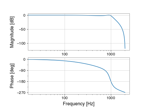
To create a low-pass filter at 1000 Hz for 4096 Hz-sampled data:

>>> from gwpy.signal.filter_design import lowpass
>>> lp = lowpass(1000, 4096)

To view the filter, you can use the BodePlot:

>>> from gwpy.plot import BodePlot
>>> plot = BodePlot(lp, sample_rate=4096)
>>> plot.show()

(png)

filter_design.highpass(sample_rate, fstop=None, gpass=2, gstop=30, type='iir', **kwargs)[source]¶

Design a high-pass filter for the given cutoff frequency

Parameters:¶

frequencyfloat

corner frequency of high-pass filter

sample_ratefloat

sampling rate of target data

fstopfloat, optional

edge-frequency of stop-band

gpassfloat, optional, default: 2

the maximum loss in the passband (dB)

gstopfloat, optional, default: 30

the minimum attenuation in the stopband (dB)

typestr, optional, default: 'iir'

the filter type, either 'iir' or 'fir'

**kwargs

other keyword arguments are passed directly to iirdesign() or firwin()

Returns:¶

filter

the formatted filter. the output format for an IIR filter depends on the input arguments, default is a tuple of (zeros, poles, gain)

Notes

By default a digital filter is returned, meaning the zeros and poles are given in the Z-domain in units of radians/sample.

Examples

To create a high-pass filter at 100 Hz for 4096 Hz-sampled data:

>>> from gwpy.signal.filter_design import highpass
>>> hp = highpass(100, 4096)

To view the filter, you can use the BodePlot:

>>> from gwpy.plot import BodePlot
>>> plot = BodePlot(hp, sample_rate=4096)
>>> plot.show()

(png)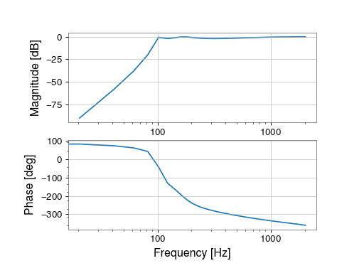

filter_design.notch(sample_rate, type='iir', output='zpk', **kwargs)[source]¶

Design a ZPK notch filter for the given frequency and sampling rate

Parameters:¶

frequencyfloat, Quantity

frequency (default in Hertz) at which to apply the notch

sample_ratefloat, Quantity

number of samples per second for TimeSeries to which this notch filter will be applied

typestr, optional, default: ‘iir’

type of filter to apply, currently only ‘iir’ is supported

outputstr, optional, default: ‘zpk’

output format for notch

**kwargs

other keyword arguments to pass to scipy.signal.iirdesign

Returns:¶

filter

the formatted filter; the output format for an IIR filter depends on the input arguments, default is a tuple of (zeros, poles, gain)

See also

scipy.signal.iirdesign

for details on the IIR filter design method and the output formats

Notes

By default a digital filter is returned, meaning the zeros and poles are given in the Z-domain in units of radians/sample.

Examples

To create a low-pass filter at 1000 Hz for 4096 Hz-sampled data:

>>> from gwpy.signal.filter_design import notch
>>> n = notch(100, 4096)

To view the filter, you can use the BodePlot:

>>> from gwpy.plot import BodePlot
>>> plot = BodePlot(n, sample_rate=4096)
>>> plot.show()

(png)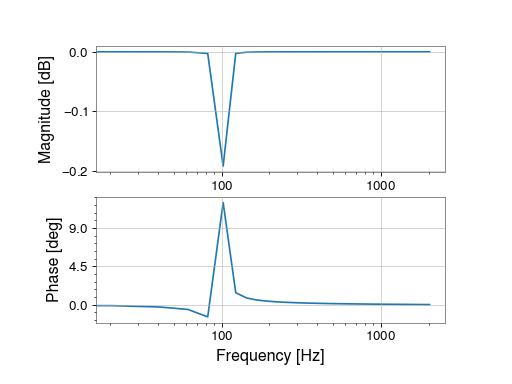

filter_design.concatenate_zpks()[source]¶

Concatenate a list of zero-pole-gain (ZPK) filters

Parameters:¶

*zpks

one or more zero-pole-gain format, each one should be a 3-tuple containing an array of zeros, an array of poles, and a gain float

Returns:¶

zerosnumpy.ndarray

the concatenated array of zeros

polesnumpy.ndarray

the concatenated array of poles

gainfloat

the overall gain

Examples

Create a lowpass and a highpass filter, and combine them:

>>> from gwpy.signal.filter_design import (
...     highpass, lowpass, concatenate_zpks)
>>> hp = highpass(100, 4096)
>>> lp = lowpass(1000, 4096)
>>> zpk = concatenate_zpks(hp, lp)

Plot the filter:

>>> from gwpy.plot import BodePlot
>>> plot = BodePlot(zpk, sample_rate=4096)
>>> plot.show()

(png)