1. Filtering a TimeSeries to detect gravitational waves
The raw ‘strain’ output of the LIGO detectors is recorded as a TimeSeries
with contributions from a large number of known and unknown noise sources,
as well as possible gravitational wave signals.
In order to uncover a real signal we need to filter out noises that otherwise
hide the signal in the data. We can do this by using the gwpy.signal
module to design a digital filter to cut out low and high frequency noise, as
well as notch out fixed frequencies polluted by known artefacts.
First we download the raw strain data from the GWOSC public archive:
from gwpy.timeseries import TimeSeries
hdata = TimeSeries.fetch_open_data('H1', 1126259446, 1126259478)
Next we can design a zero-pole-gain filter to remove the extranious noise.
First we import the gwpy.signal.filter_design module and create a
bandpass() filter to remove both low and
high frequency content
from gwpy.signal import filter_design
bp = filter_design.bandpass(50, 250, hdata.sample_rate)
Now we want to combine the bandpass with a series of
notch() filters, so we create those
for the first three harmonics of the 60 Hz AC mains power:
notches = [filter_design.notch(line, hdata.sample_rate) for
           line in (60, 120, 180)]
and concatenate each of our filters together to create a single ZPK:
zpk = filter_design.concatenate_zpks(bp, *notches)
Now, we can apply our combined filter to the data, using filtfilt=True
to filter both backwards and forwards to preserve the correct phase
at all frequencies
hfilt = hdata.filter(zpk, filtfilt=True)
Note
The filter_design methods return digital filters
by default, so we apply them using TimeSeries.filter. If we had
analogue filters (perhaps by passing analog=True to the filter design
method), the easiest application would be TimeSeries.zpk
The filter_design methods return infinite impulse
response filters by default, which, when applied, corrupt a small amount of
data at the beginning and the end of our original TimeSeries.
We can discard those data using the crop() method
(for consistency we apply this to both data series):
hdata = hdata.crop(*hdata.span.contract(1))
hfilt = hfilt.crop(*hfilt.span.contract(1))
Finally, we can plot() the original and filtered data,
adding some code to prettify the figure:
from gwpy.plot import Plot
plot = Plot(hdata, hfilt, figsize=[12, 6], separate=True, sharex=True,
            color='gwpy:ligo-hanford')
ax1, ax2 = plot.axes
ax1.set_title('LIGO-Hanford strain data around GW150914')
ax1.text(1.0, 1.01, 'Unfiltered data', transform=ax1.transAxes, ha='right')
ax1.set_ylabel('Amplitude [strain]', y=-0.2)
ax2.set_ylabel('')
ax2.text(1.0, 1.01, r'50-250\,Hz bandpass, notches at 60, 120, 180 Hz',
         transform=ax2.transAxes, ha='right')
plot.show()
(png)
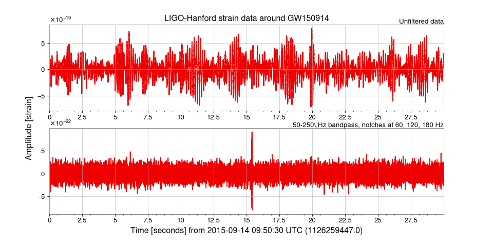
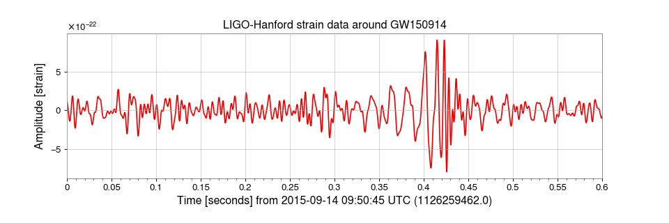
We see now a spike around 16 seconds into the data, so let’s zoom into that time (and prettify):
plot = hfilt.plot(color='gwpy:ligo-hanford')
ax = plot.gca()
ax.set_title('LIGO-Hanford strain data around GW150914')
ax.set_ylabel('Amplitude [strain]')
ax.set_xlim(1126259462, 1126259462.6)
ax.set_xscale('seconds', epoch=1126259462)
plot.show()
(png)

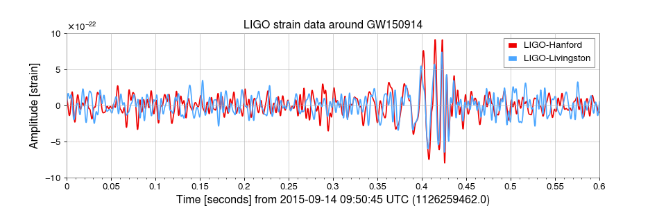
Congratulations, you have succesfully filtered LIGO data to uncover the first ever directly-detected gravitational wave signal, GW150914! But wait, what about LIGO-Livingston? We can easily add that to our figure by following the same procedure.
First, we load the new data
ldata = TimeSeries.fetch_open_data('L1', 1126259446, 1126259478)
lfilt = ldata.filter(zpk, filtfilt=True)
The article announcing the detector told us that the signals were separated by 6.9 ms between detectors, and that the relative orientation of those detectors means that we need to invert the data from one before comparing them, so we apply those corrections:
lfilt.shift('6.9ms')
lfilt *= -1
and finally make a new plot with both detectors:
plot = Plot(figsize=[12, 4])
ax = plot.gca()
ax.plot(hfilt, label='LIGO-Hanford', color='gwpy:ligo-hanford')
ax.plot(lfilt, label='LIGO-Livingston', color='gwpy:ligo-livingston')
ax.set_title('LIGO strain data around GW150914')
ax.set_xlim(1126259462, 1126259462.6)
ax.set_xscale('seconds', epoch=1126259462)
ax.set_ylabel('Amplitude [strain]')
ax.set_ylim(-1e-21, 1e-21)
ax.legend()
plot.show()
(png)

The above filtering is (almost) the same as what was applied to LIGO data to produce Figure 1 in Abbott et al. (2016) (the joint LSC-Virgo publication announcing this detection).