2. Filtering a TimeSeries with a ZPK filter
Several data streams read from the LIGO detectors are whitened before being
recorded to prevent numerical errors when using single-precision data
storage.
In this example we read such channel and undo the
whitening to show the physical content of these data.
First, we import the TimeSeries and get() the data:
from gwpy.timeseries import TimeSeries
white = TimeSeries.get(
    'L1:OAF-CAL_DARM_DQ', 'March 2 2015 12:00', 'March 2 2015 12:30')
Now, we can re-calibrate these data into displacement units by first applying
a highpass filter to remove the low-frequency noise,
and then applying our de-whitening filter in ZPK format
with five zeros at 100 Hz and five poles at 1 Hz (giving an overall DC
gain of 10 -10:
hp = white.highpass(4)
displacement = hp.zpk([100]*5, [1]*5, 1e-10)
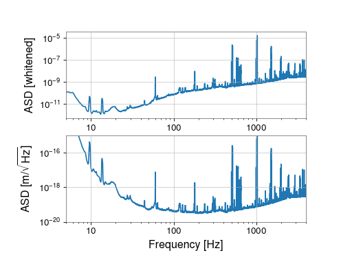
We can visualise the impact of the whitening by calculating the ASD
FrequencySeries before and after the filter,
whiteasd = white.asd(8, 4)
dispasd = displacement.asd(8, 4)
and plotting:
from gwpy.plot import Plot
plot = Plot(whiteasd, dispasd, separate=True, sharex=True,
            xscale='log', yscale='log')
Here we have passed the two
spectra in order,
then separate=True to display them on separate Axes, sharex=True to tie
the XAxis of each of the Axes
together.
Finally, we prettify our plot with some limits, and some labels:
plot.axes[0].set_ylabel('ASD [whitened]')
plot.axes[1].set_ylabel(r'ASD [m/$\sqrt{\mathrm{Hz}}$]')
plot.axes[1].set_xlabel('Frequency [Hz]')
plot.axes[1].set_ylim(1e-20, 1e-15)
plot.axes[1].set_xlim(5, 4000)
plot.show()
(png)
