4. Cross-correlating two TimeSeries
Warning
This example requires LIGO.ORG credentials for data access.
Gravitational wave detectors are very sensitive astronomical instruments, but they are also susceptible to transient noise events called _glitches_. In order to reliably detect gravitational waves and improve detector performance, we must distinguish glitches from astrophysical signals and, if possible, identify their cause.
Fortunately there are also tens of thousands of auxiliary sensors at various parts of the detector, closely monitoring mechanical subsystems and environmental conditions. We can cross-correlate data from these sensors with the primary gravitational wave data to look for evidence of terrestrial noise.
We demonstrate below a prominent ‘whistle glitch’ in the gravitational wave channel, which is also witnessed by a photodiode in the Pre-Stabilized Laser (PSL) chamber. This example uses data from the LIGO Livingston detector during Advanced LIGO’s second observing run.
First, we import the TimeSeries and get() the data:
from gwpy.timeseries import TimeSeries
hoft = TimeSeries.get('L1:GDS-CALIB_STRAIN', 1172489751, 1172489815)
aux = TimeSeries.get('L1:PSL-ISS_PDA_REL_OUT_DQ', 1172489751, 1172489815)
Next, we should whiten the data to enhance the higher-frequency
content and make a more faithful comparison between data streams.
whoft = hoft.whiten(8, 4)
waux = aux.whiten(8, 4)
We can now cross-correlate these channels:
mfilter = waux.crop(1172489782.57, 1172489783.57)
snr = whoft.correlate(mfilter).abs()
and plot the resulting normalised signal-to-noise ratio:
plot = snr.crop(1172489782.07, 1172489784.07).plot()
plot.axes[0].set_epoch(1172489783.07)
plot.axes[0].set_ylabel('Signal-to-noise ratio', fontsize=16)
plot.show()
(png)
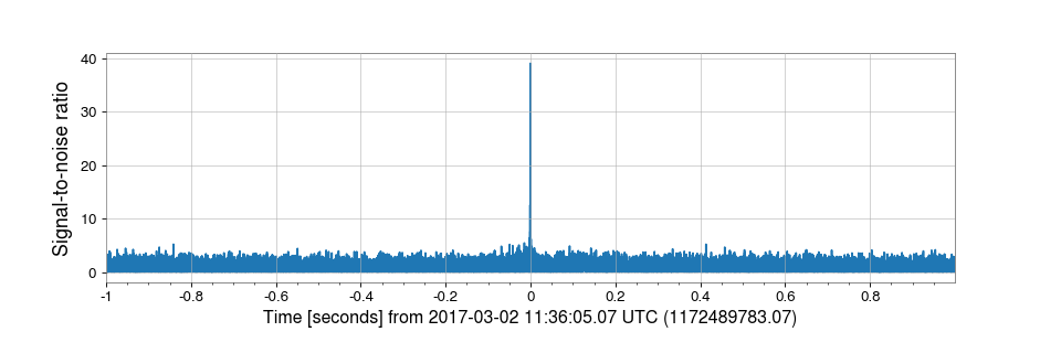
We can clearly see a loud spike (nearly SNR 40!) at GPS second 1172489783.07, which we interpret as evidence that the PSL channel is witnessing the same glitch as the gravitational wave channel.
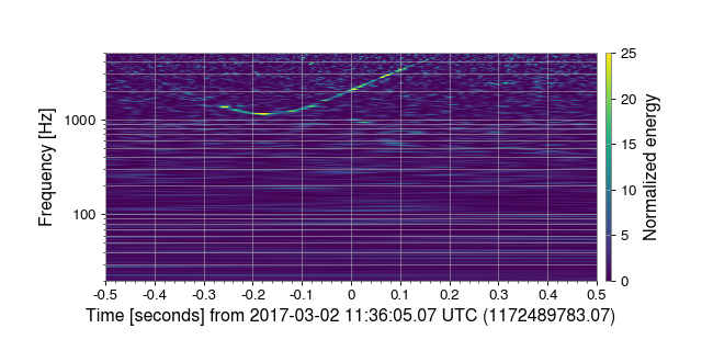
It’s now worth checking out the time-frequency morphology in both channels
using q_transform():
qhoft = whoft.q_transform(
    whiten=False,  # already white
    qrange=(4, 150),  # wider Q-transform range
    outseg=(1172489782.57, 1172489783.57),  # region of interest
)
plot = qhoft.imshow(figsize=[8, 4])
ax = plot.gca()
ax.set_xscale('seconds')
ax.set_yscale('log')
ax.set_epoch(1172489783.07)
ax.set_ylim(20, 5000)
ax.set_ylabel('Frequency [Hz]')
ax.grid(True, axis='y', which='both')
ax.colorbar(cmap='viridis', label='Normalized energy', clim=[0, 25])
plot.show()
(png)

and the same for the PSL channel:
qaux = waux.q_transform(
    whiten=False,  # already white
    qrange=(4, 150),  # wider Q-transform range
    outseg=(1172489782.57, 1172489783.57),  # region of interest
)
plot = qaux.imshow(figsize=[8, 4])
ax = plot.gca()
ax.set_xscale('seconds')
ax.set_yscale('log')
ax.set_epoch(1172489783.07)
ax.set_ylim(20, 5000)
ax.set_ylabel('Frequency [Hz]')
ax.grid(True, axis='y', which='both')
ax.colorbar(cmap='viridis', label='Normalized energy', clim=[0, 25])
plot.show()
(png)
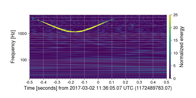
Sure enough, both channels record a clear whistle glitch at this time, although the PSL channel sees it with much greater signal energy relative to its background noise.