7. Generate the Q-transform of a `TimeSeries`¶

One of the most useful tools for filtering and visualising short-duration features in a TimeSeries is the Q-transform. This is regularly used by the Detector Characterization working groups of the LIGO Scientific Collaboration and the Virgo Collaboration to produce high-resolution time-frequency maps of transient noise (glitches) and potential gravitational-wave signals.

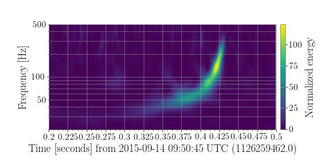
This algorithm was used to visualise the first ever gravitational-wave detection GW150914, so we can reproduce that result (bottom panel of figure 1) here.

First, we need to download the TimeSeries record for the H1 strain measurement from The Gravitational-Wave Open Science Centre (GWOSC):

from gwpy.timeseries import TimeSeries
data = TimeSeries.fetch_open_data('H1', 1126259446, 1126259478)

Next, we generate the q_transform of these data:

qspecgram = data.q_transform(outseg=(1126259462.2, 1126259462.5))

Note

We can save memory by focusing on a specific window around the interesting time. The outseg keyword argument returns a Spectrogram that is only as long as we need it to be.

Now, we can plot the resulting Spectrogram:

plot = qspecgram.plot(figsize=[8, 4])
ax = plot.gca()
ax.set_xscale('seconds')
ax.set_yscale('log')
ax.set_ylim(20, 500)
ax.set_ylabel('Frequency [Hz]')
ax.grid(True, axis='y', which='both')
ax.colorbar(cmap='viridis', label='Normalized energy')
plot.show()

(png)

Here we can clearly see the trace of a compact binary coalescence, specifically a binary black hole merger! For more details on this result, please see http://www.ligo.org/science/Publication-GW150914/.

7. Generate the Q-transform of a TimeSeries¶

7. Generate the Q-transform of a `TimeSeries`¶