1. Generating an inspiral range timeseries¶

The standard metric of the sensitivity of a gravitational-wave detector is the distance to which a canonical binary neutron star (BNS) inspiral (with two 1.4 solar mass components) would be detected with a signal-to-noise ratio (SNR) of 8.

We can estimate using gwpy.astro.inspiral_range() after calculating the power-spectral density (PSD) of the strain readout for a detector, and can plot the variation over time by looping over a power spectral density Spectrogram.

First, we need to load some data, for this we can use the LOSC public data around the GW150914 event:

from gwpy.timeseries import TimeSeries
h1 = TimeSeries.fetch_open_data('H1', 1126257414, 1126261510)
l1 = TimeSeries.fetch_open_data('L1', 1126257414, 1126261510)

and then calculating the PSD spectrogram:

h1spec = h1.spectrogram(30, fftlength=4)
l1spec = l1.spectrogram(30, fftlength=4)

To calculate the inspiral range variation, we need to create a TimeSeries in which to store the values, then loop over each PSD bin in the spectrogram, calculating the gwpy.astro.inspiral_range() for each one:

import numpy
from gwpy.astro import inspiral_range
h1range = TimeSeries(numpy.zeros(len(h1spec)),
                     dt=h1spec.dt, t0=h1spec.t0, unit='Mpc')
l1range = h1range.copy()
for i in range(h1range.size):
    h1range[i] = inspiral_range(h1spec[i], fmin=10)
    l1range[i] = inspiral_range(l1spec[i], fmin=10)

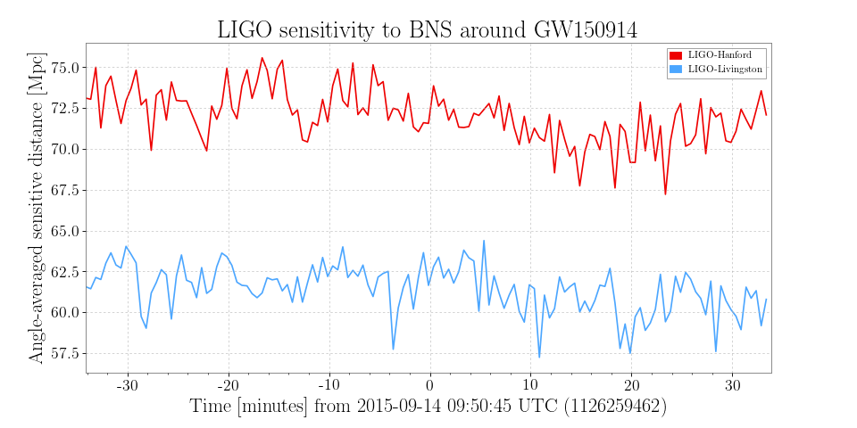
We can now easily plot the timeseries to see the variation in LIGO sensitivity over the hour or so including GW150914:

from gwpy.plotter.colors import GW_OBSERVATORY_COLORS as GWO_COLORS
plot = h1range.plot(label='LIGO-Hanford', color=GWO_COLORS['H1'])
ax = plot.gca()
ax.plot(l1range, label='LIGO-Livingston', color=GWO_COLORS['L1'])
ax.set_ylabel('Angle-averaged sensitive distance [Mpc]')
ax.set_title('LIGO sensitivity to BNS around GW150914')
ax.set_epoch(1126259462)  # <- set 0 on plot to GW150914
ax.legend()
plot.show()

(png)