2. Plotting a spectrogram of all open data for 1 day¶

In order to study interferometer performance, it is common in LIGO to plot all of the data for a day, in order to determine trends, and see data-quality issues.

This is done for the LIGO-Virgo detector network, with up-to-date plots available from the LIGO Open Science Center (LOSC).

This example demonstrates how to download data segments from LOSC, then use those to build a day-timescale spectrogram plot of LIGO-Hanford strain data.

2.1. Getting the segments¶

First, we need to fetch the Open Data timeline segments from LOSC. To do that we can call the DataQualityFlag.fetch_open_data() method using 'H1_DATA' as the flag (for an explanation of what this means, read up on The S6 Data Release).

from gwpy.segments import DataQualityFlag
h1segs = DataQualityFlag.fetch_open_data('H1_DATA',
                                         'Sep 16 2010', 'Sep 17 2010')

For sanity, lets plot these segments:

splot = h1segs.plot(figsize=[12, 3])
splot.show()

(png)

../../_images/open-data-spectrogram-2.png

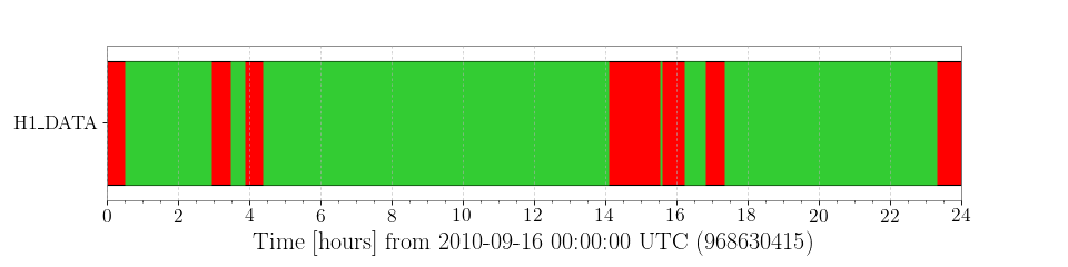
We see that the LIGO Hanford Observatory detector was operating for the majority of the day, with a few outages of ~30 minutes or so.

We can use the abs() function to display the total amount of time spent taking data:

print(abs(h1segs.active))

2.2. Working with strain data¶

Now, we can loop through the active segments of 'H1_DATA' and fetch the strain TimeSeries for each segment, calculating a Spectrogram for each segment.

from gwpy.timeseries import TimeSeries
spectrograms = []
for start, end in h1segs.active:
    h1strain = TimeSeries.fetch_open_data('H1', start, end, verbose=True)
    specgram = h1strain.spectrogram(30, fftlength=4) ** (1/2.)
    spectrograms.append(specgram)

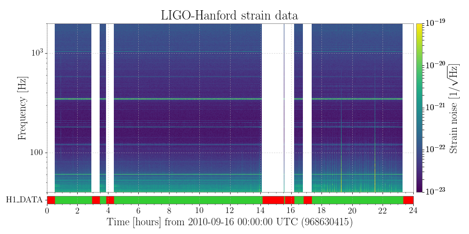
Finally, we can build a plot():

from gwpy.plotter import SpectrogramPlot
plot = SpectrogramPlot()
ax = plot.gca()
for specgram in spectrograms:
    ax.plot(specgram)
ax.set_epoch('Sep 16 2010')
ax.set_xlim('Sep 16 2010', 'Sep 17 2010')
ax.set_ylim(40, 2000)
ax.set_yscale('log')
ax.set_ylabel('Frequency [Hz]')
ax.set_title('LIGO-Hanford strain data')
plot.add_colorbar(cmap='viridis', clim=(1e-23, 1e-19), log=True,
                  label=r'Strain noise [1/\rtHz]')
plot.add_state_segments(h1segs, ax=ax)
plot.show()

(png)

../../_images/open-data-spectrogram-5.png