TimeSeries¶

class gwpy.timeseries.TimeSeries[source]¶

Bases: gwpy.timeseries.core.TimeSeriesBase

A time-domain data array.

Parameters:

value : array-like input data array unit : Unit, optional physical unit of these data t0 : LIGOTimeGPS, float, str, optional GPS epoch associated with these data, any input parsable by to_gps is fine dt : float, Quantity, optional time between successive samples (seconds), can also be given inversely via sample_rate sample_rate : float, Quantity, optional the rate of samples per second (Hertz), can also be given inversely via dt times : array-like the complete array of GPS times accompanying the data for this series. This argument takes precedence over t0 and dt so should be given in place of these if relevant, not alongside name : str, optional descriptive title for this array channel : Channel, str, optional source data stream for these data dtype : dtype, optional input data type copy : bool, optional choose to copy the input data to new memory subok : bool, optional allow passing of sub-classes by the array generator

Notes

The necessary metadata to reconstruct timing information are recorded in the epoch and sample_rate attributes. This time-stamps can be returned via the times property.

All comparison operations performed on a TimeSeries will return a StateTimeSeries - a boolean array with metadata copied from the starting TimeSeries.

Examples

>>> from gwpy.timeseries import TimeSeries

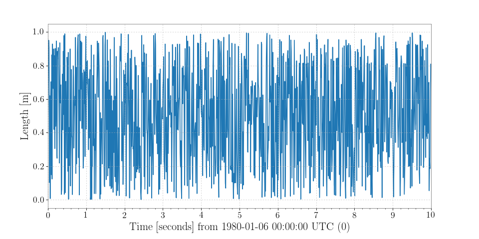
To create an array of random numbers, sampled at 100 Hz, in units of ‘metres’:

>>> from numpy import random
>>> series = TimeSeries(random.random(1000), sample_rate=100, unit='m')

which can then be simply visualised via

>>> plot = series.plot()
>>> plot.show()

(png)

Methods Summary

abs(x, /[, out, where, casting, order, …])	Calculate the absolute value element-wise.
all([axis, out, keepdims])	Returns True if all elements evaluate to True.
any([axis, out, keepdims])	Returns True if any of the elements of a evaluate to True.
append(other[, gap, inplace, pad, resize])	Connect another series onto the end of the current one.
argmax([axis, out])	Return indices of the maximum values along the given axis.
argmin([axis, out])	Return indices of the minimum values along the given axis of a.
argpartition(kth[, axis, kind, order])	Returns the indices that would partition this array.
argsort([axis, kind, order])	Returns the indices that would sort this array.
asd([fftlength, overlap, window, method])	Calculate the ASD FrequencySeries of this TimeSeries
astype(dtype[, order, casting, subok, copy])	Copy of the array, cast to a specified type.
auto_coherence(dt[, fftlength, overlap, window])	Calculate the frequency-coherence between this TimeSeries and a time-shifted copy of itself.
average_fft([fftlength, overlap, window])	Compute the averaged one-dimensional DFT of this TimeSeries.
bandpass(flow, fhigh[, gpass, gstop, fstop, …])	Filter this TimeSeries with a band-pass filter.
byteswap(inplace)	Swap the bytes of the array elements
choose(choices[, out, mode])	Use an index array to construct a new array from a set of choices.
clip([min, max, out])	Return an array whose values are limited to [min, max].
coherence(other[, fftlength, overlap, window])	Calculate the frequency-coherence between this TimeSeries and another.
coherence_spectrogram(other, stride[, …])	Calculate the coherence spectrogram between this TimeSeries and other.
compress(condition[, axis, out])	Return selected slices of this array along given axis.
conj()	Complex-conjugate all elements.
conjugate()	Return the complex conjugate, element-wise.
copy([order])	Return a copy of the array.
crop([start, end, copy])	Crop this series to the given x-axis extent.
csd(other[, fftlength, overlap, window])	Calculate the CSD FrequencySeries for two TimeSeries
csd_spectrogram(other, stride[, fftlength, …])	Calculate the cross spectral density spectrogram of this TimeSeries with ‘other’.
cumprod([axis, dtype, out])	Return the cumulative product of the elements along the given axis.
cumsum([axis, dtype, out])	Return the cumulative sum of the elements along the given axis.
decompose([bases])	Generates a new Quantity with the units decomposed.
demodulate(f[, stride, exp, deg])	Compute the average magnitude and phase of this TimeSeries once per stride at a given frequency.
detrend([detrend])	Remove the trend from this TimeSeries
diagonal([offset, axis1, axis2])	Return specified diagonals.
diff([n, axis])	Calculate the n-th order discrete difference along given axis.
dot(b[, out])	Dot product of two arrays.
dump(file)	Dump a pickle of the array to the specified file.
dumps()	Returns the pickle of the array as a string.
ediff1d([to_end, to_begin])
fetch(channel, start, end[, host, port, …])	Fetch data from NDS
fetch_open_data(ifo, start, end[, …])	Fetch open-access data from the LIGO Open Science Center
fft([nfft])	Compute the one-dimensional discrete Fourier transform of this TimeSeries.
fftgram(stride)	Calculate the Fourier-gram of this TimeSeries.
fill(value)	Fill the array with a scalar value.
filter(*filt, **kwargs)	Filter this TimeSeries with an IIR or FIR filter
find(channel, start, end[, frametype, pad, …])	Find and read data from frames for a channel
flatten([order])	Return a copy of the array collapsed into one dimension.
from_lal(lalts[, copy])	Generate a new TimeSeries from a LAL TimeSeries of any type.
from_nds2_buffer(buffer_, **metadata)	Construct a new TimeSeries from an nds2.buffer object
from_pycbc(pycbcseries[, copy])	Convert a pycbc.types.timeseries.TimeSeries into a TimeSeries
get(channel, start, end[, pad, dtype, …])	Get data for this channel from frames or NDS
getfield(dtype[, offset])	Returns a field of the given array as a certain type.
highpass(frequency[, gpass, gstop, fstop, …])	Filter this TimeSeries with a high-pass filter.
insert(obj, values[, axis])	Insert values along the given axis before the given indices and return a new Quantity object.
is_compatible(other)	Check whether this series and other have compatible metadata
is_contiguous(other[, tol])	Check whether other is contiguous with self.
item(*args)	Copy an element of an array to a standard Python scalar and return it.
itemset(*args)	Insert scalar into an array (scalar is cast to array’s dtype, if possible)
lowpass(frequency[, gpass, gstop, fstop, …])	Filter this TimeSeries with a Butterworth low-pass filter.
max([axis, out])	Return the maximum along a given axis.
mean([axis, dtype, out, keepdims])	Returns the average of the array elements along given axis.
median([axis])	Compute the median along the specified axis.
min([axis, out, keepdims])	Return the minimum along a given axis.
nansum([axis, out, keepdims])
newbyteorder([new_order])	Return the array with the same data viewed with a different byte order.
nonzero()	Return the indices of the elements that are non-zero.
notch(frequency[, type, filtfilt])	Notch out a frequency in this TimeSeries.
override_unit(unit[, parse_strict])	Forcefully reset the unit of these data
pad(pad_width, **kwargs)	Pad this series to a new size
partition(kth[, axis, kind, order])	Rearranges the elements in the array in such a way that value of the element in kth position is in the position it would be in a sorted array.
plot(**kwargs)	Plot the data for this timeseries
prepend(other[, gap, inplace, pad, resize])	Connect another series onto the start of the current one.
prod([axis, dtype, out, keepdims])	Return the product of the array elements over the given axis
psd([fftlength, overlap, window, method])	Calculate the PSD FrequencySeries for this TimeSeries
ptp([axis, out])	Peak to peak (maximum - minimum) value along a given axis.
put(indices, values[, mode])	Set a.flat[n] = values[n] for all n in indices.
q_transform([qrange, frange, gps, search, …])	Scan a TimeSeries using a multi-Q transform
ravel([order])	Return a flattened array.
rayleigh_spectrogram(stride[, fftlength, …])	Calculate the Rayleigh statistic spectrogram of this TimeSeries
rayleigh_spectrum([fftlength, overlap])	Calculate the Rayleigh FrequencySeries for this TimeSeries.
read(source, *args, **kwargs)	Read data into a TimeSeries
repeat(repeats[, axis])	Repeat elements of an array.
resample(rate[, window, ftype, n])	Resample this Series to a new rate
reshape(shape[, order])	Returns an array containing the same data with a new shape.
resize(new_shape[, refcheck])	Change shape and size of array in-place.
rms([stride])	Calculate the root-mean-square value of this TimeSeries once per stride.
round([decimals, out])	Return a with each element rounded to the given number of decimals.
searchsorted(v[, side, sorter])	Find indices where elements of v should be inserted in a to maintain order.
setfield(val, dtype[, offset])	Put a value into a specified place in a field defined by a data-type.
setflags([write, align, uic])	Set array flags WRITEABLE, ALIGNED, and UPDATEIFCOPY, respectively.
shift(delta)	Shift this TimeSeries forward in time by delta
sort([axis, kind, order])	Sort an array, in-place.
spectral_variance(stride[, fftlength, …])	Calculate the SpectralVariance of this TimeSeries.
spectrogram(stride[, fftlength, overlap, …])	Calculate the average power spectrogram of this TimeSeries using the specified average spectrum method.
spectrogram2(fftlength[, overlap])	Calculate the non-averaged power Spectrogram of this TimeSeries
squeeze([axis])	Remove single-dimensional entries from the shape of a.
std([axis, dtype, out, ddof, keepdims])	Returns the standard deviation of the array elements along given axis.
sum([axis, dtype, out, keepdims])	Return the sum of the array elements over the given axis.
swapaxes(axis1, axis2)	Return a view of the array with axis1 and axis2 interchanged.
take(indices[, axis, out, mode])	Return an array formed from the elements of a at the given indices.
to(unit[, equivalencies])	Return a new Quantity object with the specified unit.
to_lal()	Convert this TimeSeries into a LAL TimeSeries.
to_pycbc([copy])	Convert this TimeSeries into a PyCBC
to_value([unit, equivalencies])	The numerical value, possibly in a different unit.
tobytes([order])	Construct Python bytes containing the raw data bytes in the array.
tofile(fid[, sep, format])	Write array to a file as text or binary (default).
tolist()	Return the array as a (possibly nested) list.
tostring([order])	Construct Python bytes containing the raw data bytes in the array.
trace([offset, axis1, axis2, dtype, out])	Return the sum along diagonals of the array.
transpose(*axes)	Returns a view of the array with axes transposed.
update(other[, inplace])	Update this series by appending new data from an other and dropping the same amount of data off the start.
value_at(x)	Return the value of this Series at the given xindex value
var([axis, dtype, out, ddof, keepdims])	Returns the variance of the array elements, along given axis.
view([dtype, type])	New view of array with the same data.
whiten(fftlength[, overlap, method, window, …])	White this TimeSeries against its own ASD
write(target, *args, **kwargs)	Write this TimeSeries to a file
zip()	Zip the xindex and value arrays of this Series
zpk(zeros, poles, gain[, analog])	Filter this TimeSeries by applying a zero-pole-gain filter

Methods Documentation

abs(x, /, out=None, *, where=True, casting='same_kind', order='K', dtype=None, subok=True[, signature, extobj])[source]¶

Calculate the absolute value element-wise.

Parameters:

x : array_like Input array. out : ndarray, None, or tuple of ndarray and None, optional A location into which the result is stored. If provided, it must have a shape that the inputs broadcast to. If not provided or None, a freshly-allocated array is returned. A tuple (possible only as a keyword argument) must have length equal to the number of outputs. where : array_like, optional Values of True indicate to calculate the ufunc at that position, values of False indicate to leave the value in the output alone. **kwargs For other keyword-only arguments, see the ufunc docs.

Returns:

absolute : ndarray An ndarray containing the absolute value of each element in x. For complex input, a + ib, the absolute value is System Message: WARNING/2 (\sqrt{ a^2 + b^2 }) latex exited with error [stdout] This is pdfTeX, Version 3.1415926-2.5-1.40.14 (TeX Live 2013) restricted \write18 enabled. entering extended mode (./math.tex LaTeX2e <2011/06/27> Babel <v3.8m> and hyphenation patterns for english, dumylang, nohyphenation, lo aded. (/usr/share/texlive/texmf-dist/tex/latex/base/article.cls Document Class: article 2007/10/19 v1.4h Standard LaTeX document class (/usr/share/texlive/texmf-dist/tex/latex/base/size12.clo)) (/usr/share/texlive/texmf-dist/tex/latex/base/inputenc.sty (/usr/share/texlive/texmf-dist/tex/latex/ucs/utf8x.def)) (/usr/share/texlive/texmf-dist/tex/latex/ucs/ucs.sty (/usr/share/texlive/texmf-dist/tex/latex/ucs/data/uni-global.def)) (/usr/share/texlive/texmf-dist/tex/latex/amsmath/amsmath.sty For additional information on amsmath, use the `?' option. (/usr/share/texlive/texmf-dist/tex/latex/amsmath/amstext.sty (/usr/share/texlive/texmf-dist/tex/latex/amsmath/amsgen.sty)) (/usr/share/texlive/texmf-dist/tex/latex/amsmath/amsbsy.sty) (/usr/share/texlive/texmf-dist/tex/latex/amsmath/amsopn.sty)) (/usr/share/texlive/texmf-dist/tex/latex/amscls/amsthm.sty) (/usr/share/texlive/texmf-dist/tex/latex/amsfonts/amssymb.sty (/usr/share/texlive/texmf-dist/tex/latex/amsfonts/amsfonts.sty)) ! LaTeX Error: File `anyfontsize.sty' not found. Type X to quit or <RETURN> to proceed, or enter new name. (Default extension: sty) Enter file name: ! Emergency stop. <read *> l.9 \usepackage {bm}^^M No pages of output. Transcript written on math.log. .

Examples

>>> x = np.array([-1.2, 1.2])
>>> np.absolute(x)
array([ 1.2,  1.2])
>>> np.absolute(1.2 + 1j)
1.5620499351813308

Plot the function over [-10, 10]:

>>> import matplotlib.pyplot as plt

>>> x = np.linspace(start=-10, stop=10, num=101)
>>> plt.plot(x, np.absolute(x))
>>> plt.show()

(png)

Plot the function over the complex plane:

>>> xx = x + 1j * x[:, np.newaxis]
>>> plt.imshow(np.abs(xx), extent=[-10, 10, -10, 10], cmap='gray')
>>> plt.show()

(png)

all(axis=None, out=None, keepdims=False)¶

Returns True if all elements evaluate to True.

Refer to numpy.all for full documentation.

See also

numpy.all

equivalent function

any(axis=None, out=None, keepdims=False)¶

Returns True if any of the elements of a evaluate to True.

Refer to numpy.any for full documentation.

See also

numpy.any

equivalent function

append(other, gap='raise', inplace=True, pad=0, resize=True)[source]¶

Connect another series onto the end of the current one.

Parameters:

other : Series another series of the same type to connect to this one gap : str, optional, default: 'raise' action to perform if there’s a gap between the other series and this one. One of 'raise' - raise an Exception 'ignore' - remove gap and join data 'pad' - pad gap with zeros inplace : bool, optional, default: True perform operation in-place, modifying current Series, otherwise copy data and return new Series Warning inplace append bypasses the reference check in numpy.ndarray.resize, so be carefully to only use this for arrays that haven’t been sharing their memory! pad : float, optional, default: 0.0 value with which to pad discontiguous series resize : bool, optional, default: True resize this array to accommodate new data, otherwise shift the old data to the left (potentially falling off the start) and put the new data in at the end

Returns:

series : Series a new series containing joined data sets

argmax(axis=None, out=None)¶

Return indices of the maximum values along the given axis.

Refer to numpy.argmax for full documentation.

See also

numpy.argmax

equivalent function

argmin(axis=None, out=None)¶

Return indices of the minimum values along the given axis of a.

Refer to numpy.argmin for detailed documentation.

See also

numpy.argmin

equivalent function

argpartition(kth, axis=-1, kind='introselect', order=None)¶

Returns the indices that would partition this array.

Refer to numpy.argpartition for full documentation.

New in version 1.8.0.

See also

numpy.argpartition

equivalent function

argsort(axis=-1, kind='quicksort', order=None)¶

Returns the indices that would sort this array.

Refer to numpy.argsort for full documentation.

See also

numpy.argsort

equivalent function

asd(fftlength=None, overlap=None, window='hann', method='scipy-welch', **kwargs)[source]¶

Calculate the ASD FrequencySeries of this TimeSeries

Parameters:

fftlength : float number of seconds in single FFT, defaults to a single FFT covering the full duration overlap : float, optional number of seconds of overlap between FFTs, defaults to the recommended overlap for the given window (if given), or 0 window : str, numpy.ndarray, optional window function to apply to timeseries prior to FFT, see scipy.signal.get_window() for details on acceptable formats method : str, optional FFT-averaging method, default: 'scipy-welch', see Notes for more details

Returns:

psd : FrequencySeries a data series containing the PSD.

See also

TimeSeries.psd

Notes

The available methods are:

Method name	Function
welch	gwpy.signal.fft.basic.welch
bartlett	gwpy.signal.fft.basic.bartlett
median	gwpy.signal.fft.basic.median
median_mean	gwpy.signal.fft.basic.median_mean
pycbc_welch	gwpy.signal.fft.pycbc.welch
pycbc_bartlett	gwpy.signal.fft.pycbc.bartlett
pycbc_median	gwpy.signal.fft.pycbc.median
pycbc_median_mean	gwpy.signal.fft.pycbc.median_mean
lal_welch	gwpy.signal.fft.lal.welch
lal_bartlett	gwpy.signal.fft.lal.bartlett
lal_median	gwpy.signal.fft.lal.median
lal_median_mean	gwpy.signal.fft.lal.median_mean
scipy_welch	gwpy.signal.fft.scipy.welch
scipy_bartlett	gwpy.signal.fft.scipy.bartlett

See FFT routines for GWpy for more details

astype(dtype, order='K', casting='unsafe', subok=True, copy=True)¶

Copy of the array, cast to a specified type.

Parameters:	dtype : str or dtype Typecode or data-type to which the array is cast. order : {‘C’, ‘F’, ‘A’, ‘K’}, optional Controls the memory layout order of the result. ‘C’ means C order, ‘F’ means Fortran order, ‘A’ means ‘F’ order if all the arrays are Fortran contiguous, ‘C’ order otherwise, and ‘K’ means as close to the order the array elements appear in memory as possible. Default is ‘K’. casting : {‘no’, ‘equiv’, ‘safe’, ‘same_kind’, ‘unsafe’}, optional Controls what kind of data casting may occur. Defaults to ‘unsafe’ for backwards compatibility. ‘no’ means the data types should not be cast at all. ‘equiv’ means only byte-order changes are allowed. ‘safe’ means only casts which can preserve values are allowed. ‘same_kind’ means only safe casts or casts within a kind, like float64 to float32, are allowed. ‘unsafe’ means any data conversions may be done. subok : bool, optional If True, then sub-classes will be passed-through (default), otherwise the returned array will be forced to be a base-class array. copy : bool, optional By default, astype always returns a newly allocated array. If this is set to false, and the dtype, order, and subok requirements are satisfied, the input array is returned instead of a copy.
Returns:	arr_t : ndarray Unless copy is False and the other conditions for returning the input array are satisfied (see description for copy input parameter), arr_t is a new array of the same shape as the input array, with dtype, order given by dtype, order.
Raises:	ComplexWarning When casting from complex to float or int. To avoid this, one should use a.real.astype(t).

Notes

Starting in NumPy 1.9, astype method now returns an error if the string dtype to cast to is not long enough in ‘safe’ casting mode to hold the max value of integer/float array that is being casted. Previously the casting was allowed even if the result was truncated.

Examples

>>> x = np.array([1, 2, 2.5])
>>> x
array([ 1. ,  2. ,  2.5])

>>> x.astype(int)
array([1, 2, 2])

auto_coherence(dt, fftlength=None, overlap=None, window='hann', **kwargs)[source]¶

Calculate the frequency-coherence between this TimeSeries and a time-shifted copy of itself.

The standard TimeSeries.coherence() is calculated between the input TimeSeries and a cropped copy of itself. Since the cropped version will be shorter, the input series will be shortened to match.

Parameters:

dt : float duration (in seconds) of time-shift fftlength : float, optional number of seconds in single FFT, defaults to a single FFT covering the full duration overlap : float, optional number of seconds of overlap between FFTs, defaults to the recommended overlap for the given window (if given), or 0 window : str, numpy.ndarray, optional window function to apply to timeseries prior to FFT, see scipy.signal.get_window() for details on acceptable formats **kwargs any other keyword arguments accepted by matplotlib.mlab.cohere() except NFFT, window, and noverlap which are superceded by the above keyword arguments

Returns:

coherence : FrequencySeries the coherence FrequencySeries of this TimeSeries with the other

See also

matplotlib.mlab.cohere()

for details of the coherence calculator

Notes

The TimeSeries.auto_coherence() will perform best when dt is approximately fftlength / 2.

average_fft(fftlength=None, overlap=0, window=None)[source]¶

Compute the averaged one-dimensional DFT of this TimeSeries.

This method computes a number of FFTs of duration fftlength and overlap (both given in seconds), and returns the mean average. This method is analogous to the Welch average method for power spectra.

Parameters:	fftlength : float number of seconds in single FFT, default, use whole TimeSeries overlap : float, optional number of seconds of overlap between FFTs, defaults to the recommended overlap for the given window (if given), or 0 window : str, numpy.ndarray, optional window function to apply to timeseries prior to FFT, see scipy.signal.get_window() for details on acceptable formats
Returns:	out : complex-valued FrequencySeries the transformed output, with populated frequencies array metadata

See also

scipy.fftpack, used.

bandpass(flow, fhigh, gpass=2, gstop=30, fstop=None, type='iir', filtfilt=True, **kwargs)[source]¶

Filter this TimeSeries with a band-pass filter.

Parameters:

flow : float lower corner frequency of pass band fhigh : float upper corner frequency of pass band gpass : float the maximum loss in the passband (dB). gstop : float the minimum attenuation in the stopband (dB). fstop : tuple of float, optional (low, high) edge-frequencies of stop band type : str the filter type, either 'iir' or 'fir' **kwargs other keyword arguments are passed to gwpy.signal.filter_design.bandpass()

Returns:

bpseries : TimeSeries a band-passed version of the input TimeSeries

See also

gwpy.signal.filter_design.bandpass

for details on the filter design

TimeSeries.filter

for details on how the filter is applied

When using scipy < 0.16.0 some higher-order filters may be unstable. With scipy >= 0.16.0 higher-order filters are decomposed into second-order-sections, and so are much more stable.

byteswap(inplace)¶

Swap the bytes of the array elements

Toggle between low-endian and big-endian data representation by returning a byteswapped array, optionally swapped in-place.

Parameters:	inplace : bool, optional If True, swap bytes in-place, default is False.
Returns:	out : ndarray The byteswapped array. If inplace is True, this is a view to self.

Examples

>>> A = np.array([1, 256, 8755], dtype=np.int16)
>>> map(hex, A)
['0x1', '0x100', '0x2233']
>>> A.byteswap(True)
array([  256,     1, 13090], dtype=int16)
>>> map(hex, A)
['0x100', '0x1', '0x3322']

Arrays of strings are not swapped

>>> A = np.array(['ceg', 'fac'])
>>> A.byteswap()
array(['ceg', 'fac'],
      dtype='|S3')

choose(choices, out=None, mode='raise')¶

Use an index array to construct a new array from a set of choices.

Refer to numpy.choose for full documentation.

See also

numpy.choose

equivalent function

clip(min=None, max=None, out=None)¶

Return an array whose values are limited to [min, max]. One of max or min must be given.

Refer to numpy.clip for full documentation.

See also

numpy.clip

equivalent function

coherence(other, fftlength=None, overlap=None, window='hann', **kwargs)[source]¶

Calculate the frequency-coherence between this TimeSeries and another.

Parameters:

other : TimeSeries TimeSeries signal to calculate coherence with fftlength : float, optional number of seconds in single FFT, defaults to a single FFT covering the full duration overlap : float, optional number of seconds of overlap between FFTs, defaults to the recommended overlap for the given window (if given), or 0 window : str, numpy.ndarray, optional window function to apply to timeseries prior to FFT, see scipy.signal.get_window() for details on acceptable formats **kwargs any other keyword arguments accepted by matplotlib.mlab.cohere() except NFFT, window, and noverlap which are superceded by the above keyword arguments

Returns:

coherence : FrequencySeries the coherence FrequencySeries of this TimeSeries with the other

See also

matplotlib.mlab.cohere()

for details of the coherence calculator

Notes

If self and other have difference TimeSeries.sample_rate values, the higher sampled TimeSeries will be down-sampled to match the lower.

coherence_spectrogram(other, stride, fftlength=None, overlap=None, window='hann', nproc=1)[source]¶

Calculate the coherence spectrogram between this TimeSeries and other.

Parameters:

other : TimeSeries the second TimeSeries in this CSD calculation stride : float number of seconds in single PSD (column of spectrogram) fftlength : float number of seconds in single FFT overlap : float, optional number of seconds of overlap between FFTs, defaults to the recommended overlap for the given window (if given), or 0 window : str, numpy.ndarray, optional window function to apply to timeseries prior to FFT, see scipy.signal.get_window() for details on acceptable formats nproc : int number of parallel processes to use when calculating individual coherence spectra.

Returns:

spectrogram : Spectrogram time-frequency coherence spectrogram as generated from the input time-series.

compress(condition, axis=None, out=None)¶

Return selected slices of this array along given axis.

Refer to numpy.compress for full documentation.

See also

numpy.compress

equivalent function

conj()¶

Complex-conjugate all elements.

Refer to numpy.conjugate for full documentation.

See also

numpy.conjugate

equivalent function

conjugate()¶

Return the complex conjugate, element-wise.

Refer to numpy.conjugate for full documentation.

See also

numpy.conjugate

equivalent function

copy(order='C')[source]¶

Return a copy of the array.

Parameters:	order : {‘C’, ‘F’, ‘A’, ‘K’}, optional Controls the memory layout of the copy. ‘C’ means C-order, ‘F’ means F-order, ‘A’ means ‘F’ if a is Fortran contiguous, ‘C’ otherwise. ‘K’ means match the layout of a as closely as possible. (Note that this function and :func:numpy.copy are very similar, but have different default values for their order= arguments.)

See also

numpy.copy, numpy.copyto

Examples

>>> x = np.array([[1,2,3],[4,5,6]], order='F')

>>> y = x.copy()

>>> x.fill(0)

>>> x
array([[0, 0, 0],
       [0, 0, 0]])

>>> y
array([[1, 2, 3],
       [4, 5, 6]])

>>> y.flags['C_CONTIGUOUS']
True

crop(start=None, end=None, copy=False)[source]¶

Crop this series to the given x-axis extent.

Parameters:	start : float, optional lower limit of x-axis to crop to, defaults to current x0 end : float, optional upper limit of x-axis to crop to, defaults to current series end copy : bool, optional, default: False copy the input data to fresh memory, otherwise return a view
Returns:	series : Series A new series with a sub-set of the input data

Notes

If either start or end are outside of the original Series span, warnings will be printed and the limits will be restricted to the xspan

csd(other, fftlength=None, overlap=None, window='hann', **kwargs)[source]¶

Calculate the CSD FrequencySeries for two TimeSeries

Parameters:

other : TimeSeries the second TimeSeries in this CSD calculation fftlength : float number of seconds in single FFT, defaults to a single FFT covering the full duration overlap : float, optional number of seconds of overlap between FFTs, defaults to the recommended overlap for the given window (if given), or 0 window : str, numpy.ndarray, optional window function to apply to timeseries prior to FFT, see scipy.signal.get_window() for details on acceptable formats

Returns:

csd : FrequencySeries a data series containing the CSD.

csd_spectrogram(other, stride, fftlength=None, overlap=0, window='hann', nproc=1, **kwargs)[source]¶

Calculate the cross spectral density spectrogram of this

TimeSeries with ‘other’.

Parameters:

other : TimeSeries second time-series for cross spectral density calculation stride : float number of seconds in single PSD (column of spectrogram). fftlength : float number of seconds in single FFT. overlap : float, optional number of seconds of overlap between FFTs, defaults to the recommended overlap for the given window (if given), or 0 window : str, numpy.ndarray, optional window function to apply to timeseries prior to FFT, see scipy.signal.get_window() for details on acceptable formats nproc : int maximum number of independent frame reading processes, default is set to single-process file reading.

Returns:

spectrogram : Spectrogram time-frequency cross spectrogram as generated from the two input time-series.

cumprod(axis=None, dtype=None, out=None)¶

Return the cumulative product of the elements along the given axis.

Refer to numpy.cumprod for full documentation.

See also

numpy.cumprod

equivalent function

cumsum(axis=None, dtype=None, out=None)¶

Return the cumulative sum of the elements along the given axis.

Refer to numpy.cumsum for full documentation.

See also

numpy.cumsum

equivalent function

decompose(bases=[])¶

Generates a new Quantity with the units decomposed. Decomposed units have only irreducible units in them (see astropy.units.UnitBase.decompose).

Parameters:	bases : sequence of UnitBase, optional The bases to decompose into. When not provided, decomposes down to any irreducible units. When provided, the decomposed result will only contain the given units. This will raises a UnitsError if it’s not possible to do so.
Returns:	newq : Quantity A new object equal to this quantity with units decomposed.

demodulate(f, stride=1, exp=False, deg=True)[source]¶

Compute the average magnitude and phase of this TimeSeries

once per stride at a given frequency.

Parameters:	f : float frequency (Hz) at which to demodulate the signal stride : float, optional stride (seconds) between calculations, defaults to 1 second exp : bool, optional return the demodulated magnitude and phase trends as one TimeSeries object representing a complex exponential deg : bool, optional if exp=False, calculates the phase in degrees
Returns:	mag, phase : TimeSeries if exp=False, returns a pair of TimeSeries objects representing magnitude and phase trends with dt=stride out : TimeSeries if exp=True, returns a single TimeSeries with magnitude and phase trends represented as mag * exp(1j*phase) with dt=stride

Examples

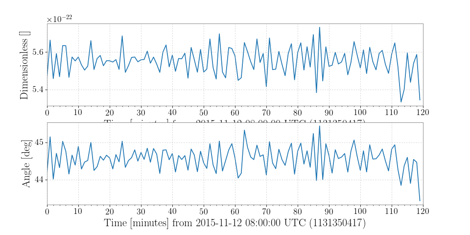
Demodulation is useful when trying to examine steady sinusoidal signals we know to be contained within data. For instance, we can download some data from LOSC to look at trends of the amplitude and phase of Livingston’s calibration line at 331.3 Hz:

>>> from gwpy.timeseries import TimeSeries
>>> data = TimeSeries.fetch_open_data('L1', 1131350417, 1131357617)

We can demodulate the TimeSeries at 331.3 Hz with a stride of once per minute:

>>> amp, phase = data.demodulate(331.3, stride=60)

We can then plot these trends to visualize changes in the amplitude and phase of the calibration line:

>>> from gwpy.plotter import TimeSeriesPlot
>>> plot = TimeSeriesPlot(amp, phase, sep=True)
>>> plot.show()

(png)

detrend(detrend='constant')[source]¶

Remove the trend from this TimeSeries

This method just wraps scipy.signal.detrend() to return an object of the same type as the input.

Parameters:	detrend : str, optional the type of detrending.
Returns:	detrended : TimeSeries the detrended input series

See also

scipy.signal.detrend

for details on the options for the detrend argument, and how the operation is done

diagonal(offset=0, axis1=0, axis2=1)¶

Return specified diagonals. In NumPy 1.9 the returned array is a read-only view instead of a copy as in previous NumPy versions. In a future version the read-only restriction will be removed.

Refer to numpy.diagonal() for full documentation.

See also

numpy.diagonal

equivalent function

diff(n=1, axis=-1)[source]¶

Calculate the n-th order discrete difference along given axis.

The first order difference is given by out[n] = a[n+1] - a[n] along the given axis, higher order differences are calculated by using diff recursively.

Parameters:	n : int, optional The number of times values are differenced. axis : int, optional The axis along which the difference is taken, default is the last axis.
Returns:	diff : Series The n order differences. The shape of the output is the same as the input, except along axis where the dimension is smaller by n.

See also

numpy.diff

for documentation on the underlying method

dot(b, out=None)¶

Dot product of two arrays.

Refer to numpy.dot for full documentation.

See also

numpy.dot

equivalent function

Examples

>>> a = np.eye(2)
>>> b = np.ones((2, 2)) * 2
>>> a.dot(b)
array([[ 2.,  2.],
       [ 2.,  2.]])

This array method can be conveniently chained:

>>> a.dot(b).dot(b)
array([[ 8.,  8.],
       [ 8.,  8.]])

dump(file)¶

Dump a pickle of the array to the specified file. The array can be read back with pickle.load or numpy.load.

Parameters:	file : str A string naming the dump file.

dumps()[source]¶

Returns the pickle of the array as a string. pickle.loads or numpy.loads will convert the string back to an array.

Parameters:	None

ediff1d(to_end=None, to_begin=None)¶

fetch(channel, start, end, host=None, port=None, verbose=False, connection=None, verify=False, pad=None, allow_tape=None, type=None, dtype=None)[source]¶

Fetch data from NDS

Parameters:

channel : str, Channel the data channel for which to query start : LIGOTimeGPS, float, str GPS start time of required data, any input parseable by to_gps is fine end : LIGOTimeGPS, float, str GPS end time of required data, any input parseable by to_gps is fine host : str, optional URL of NDS server to use, if blank will try any server (in a relatively sensible order) to get the data port : int, optional port number for NDS server query, must be given with host verify : bool, optional, default: False check channels exist in database before asking for data connection : nds2.connection, optional open NDS connection to use verbose : bool, optional print verbose output about NDS progress, useful for debugging type : int, optional NDS2 channel type integer dtype : type, numpy.dtype, str, optional identifier for desired output data type

fetch_open_data(ifo, start, end, sample_rate=4096, tag=None, version=None, format=None, host='https://losc.ligo.org', verbose=False, cache=None, **kwargs)[source]¶

Fetch open-access data from the LIGO Open Science Center

Parameters:

ifo : str the two-character prefix of the IFO in which you are interested, e.g. 'L1' start : LIGOTimeGPS, float, str, optional GPS start time of required data, defaults to start of data found; any input parseable by to_gps is fine end : LIGOTimeGPS, float, str, optional GPS end time of required data, defaults to end of data found; any input parseable by to_gps is fine sample_rate : float, optional, the sample rate of desired data; most data are stored by LOSC at 4096 Hz, however there may be event-related data releases with a 16384 Hz rate, default: 4096 tag : str, optional file tag, e.g. 'CLN' to select cleaned data, or 'C00' for ‘raw’ calibrated data. version : int, optional version of files to download, defaults to highest discovered version format : str, optional the data format to download and parse, defaults to the most efficient option based on third-party libraries available; one of: 'txt.gz' - requires numpy 'hdf5' - requires h5py 'gwf' - requires LDAStools.frameCPP host : str, optional HTTP host name of LOSC server to access verbose : bool, optional, default: False print verbose output while fetching data cache : bool, optional save/read a local copy of the remote URL, default: False; useful if the same remote data are to be accessed multiple times. Set GWPY_CACHE=1 in the environment to auto-cache. **kwargs any other keyword arguments are passed to the TimeSeries.read method that parses the file that was downloaded

Notes

StateVector data are not available in txt.gz format.

Examples

>>> from gwpy.timeseries import (TimeSeries, StateVector)
>>> print(TimeSeries.fetch_open_data('H1', 1126259446, 1126259478))
TimeSeries([  2.17704028e-19,  2.08763900e-19,  2.39681183e-19,
            ...,   3.55365541e-20,  6.33533516e-20,
              7.58121195e-20]
           unit: Unit(dimensionless),
           t0: 1126259446.0 s,
           dt: 0.000244140625 s,
           name: Strain,
           channel: None)
>>> print(StateVector.fetch_open_data('H1', 1126259446, 1126259478))
StateVector([127,127,127,127,127,127,127,127,127,127,127,127,
             127,127,127,127,127,127,127,127,127,127,127,127,
             127,127,127,127,127,127,127,127]
            unit: Unit(dimensionless),
            t0: 1126259446.0 s,
            dt: 1.0 s,
            name: Data quality,
            channel: None,
            bits: Bits(0: data present
                       1: passes cbc CAT1 test
                       2: passes cbc CAT2 test
                       3: passes cbc CAT3 test
                       4: passes burst CAT1 test
                       5: passes burst CAT2 test
                       6: passes burst CAT3 test,
                       channel=None,
                       epoch=1126259446.0))

For the StateVector, the naming of the bits will be format-dependent, because they are recorded differently by LOSC in different formats.

For events published in O2 and later, LOSC typically provides multiple data sets containing the original ('C00') and cleaned ('CLN') data. To select both data sets and plot a comparison, for example:

>>> orig = TimeSeries.fetch_open_data('H1', 1187008870, 1187008896,
...                                   tag='C00')
>>> cln = TimeSeries.fetch_open_data('H1', 1187008870, 1187008896,
...                                  tag='CLN')
>>> origasd = orig.asd(fftlength=4, overlap=2)
>>> clnasd = cln.asd(fftlength=4, overlap=2)
>>> plot = origasd.plot(label='Un-cleaned')
>>> ax = plot.gca()
>>> ax.plot(clnasd, label='Cleaned')
>>> ax.set_xlim(10, 1400)
>>> ax.set_ylim(1e-24, 1e-20)
>>> ax.legend()
>>> plot.show()

(png)

fft(nfft=None)[source]¶

Compute the one-dimensional discrete Fourier transform of this TimeSeries.

Parameters:	nfft : int, optional length of the desired Fourier transform, input will be cropped or padded to match the desired length. If nfft is not given, the length of the TimeSeries will be used
Returns:	out : FrequencySeries the normalised, complex-valued FFT FrequencySeries.

See also

scipy.fftpack, used.

Notes

This method, in constrast to the numpy.fft.rfft() method it calls, applies the necessary normalisation such that the amplitude of the output FrequencySeries is correct.

fftgram(stride)[source]¶

Calculate the Fourier-gram of this TimeSeries.

At every stride, a single, complex FFT is calculated.

Parameters:	stride : float number of seconds in single PSD (column of spectrogram)
Returns:	fftgram : Spectrogram a Fourier-gram

fill(value)¶

Fill the array with a scalar value.

Parameters:	value : scalar All elements of a will be assigned this value.

Examples

>>> a = np.array([1, 2])
>>> a.fill(0)
>>> a
array([0, 0])
>>> a = np.empty(2)
>>> a.fill(1)
>>> a
array([ 1.,  1.])

filter(*filt, **kwargs)[source]¶

Filter this TimeSeries with an IIR or FIR filter

Parameters:	*filt : filter arguments 1, 2, 3, or 4 arguments defining the filter to be applied, an Nx1 ndarray of FIR coefficients an Nx6 ndarray of SOS coefficients (numerator, denominator) polynomials (zeros, poles, gain) (A, B, C, D) ‘state-space’ representation filtfilt : bool, optional filter forward and backwards to preserve phase, default: False analog : bool, optional if True, filter coefficients will be converted from Hz to Z-domain digital representation, default: False inplace : bool, optional if True, this array will be overwritten with the filtered version, default: False **kwargs other keyword arguments are passed to the filter method
Returns:	result : TimeSeries the filtered version of the input TimeSeries
Raises:	ValueError if filt arguments cannot be interpreted properly

See also

scipy.signal.sosfilt

for details on filtering with second-order sections (scipy >= 0.16 only)

scipy.signal.sosfiltfilt

for details on forward-backward filtering with second-order sections (scipy >= 0.16 only)

scipy.signal.lfilter

for details on filtering (without SOS)

scipy.signal.filtfilt

for details on forward-backward filtering (without SOS)

Notes

IIR filters are converted either into cascading second-order sections (if scipy >= 0.16 is installed), or into the (numerator, denominator) representation before being applied to this TimeSeries.

Note

When using scipy < 0.16 some higher-order filters may be unstable. With scipy >= 0.16 higher-order filters are decomposed into second-order-sections, and so are much more stable.

FIR filters are passed directly to scipy.signal.lfilter() or scipy.signal.filtfilt() without any conversions.

Examples

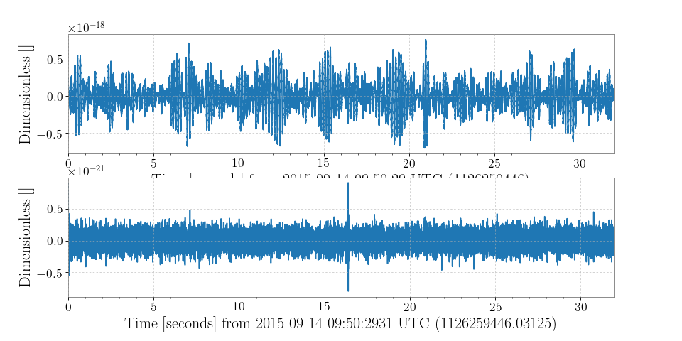
We can design an arbitrarily complicated filter using gwpy.signal.filter_design

>>> from gwpy.signal import filter_design
>>> bp = filter_design.bandpass(50, 250, 4096.)
>>> notches = [filter_design.notch(f, 4096.) for f in (60, 120, 180)]
>>> zpk = filter_design.concatenate_zpks(bp, *notches)

And then can download some data from LOSC to apply it using TimeSeries.filter:

>>> from gwpy.timeseries import TimeSeries
>>> data = TimeSeries.fetch_open_data('H1', 1126259446, 1126259478)
>>> filtered = data.filter(zpk, filtfilt=True)

We can plot the original signal, and the filtered version, cutting off either end of the filtered data to remove filter-edge artefacts

>>> from gwpy.plotter import TimeSeriesPlot
>>> plot = TimeSeriesPlot(data, filtered[128:-128], sep=True)
>>> plot.show()

(png)

find(channel, start, end, frametype=None, pad=None, dtype=None, nproc=1, verbose=False, **readargs)[source]¶

Find and read data from frames for a channel

Parameters:

channel : str, Channel the name of the channel to read, or a Channel object. start : LIGOTimeGPS, float, str GPS start time of required data, any input parseable by to_gps is fine end : LIGOTimeGPS, float, str GPS end time of required data, any input parseable by to_gps is fine frametype : str, optional name of frametype in which this channel is stored, will search for containing frame types if necessary pad : float, optional value with which to fill gaps in the source data, only used if gap is not given, or gap='pad' is given nproc : int, optional, default: 1 number of parallel processes to use, serial process by default. dtype : numpy.dtype, str, type, or dict numeric data type for returned data, e.g. numpy.float, or dict of (channel, dtype) pairs allow_tape : bool, optional, default: True allow reading from frame files on (slow) magnetic tape verbose : bool, optional print verbose output about NDS progress. **readargs any other keyword arguments to be passed to read()

flatten(order='C')¶

Return a copy of the array collapsed into one dimension.

Parameters:	order : {‘C’, ‘F’, ‘A’, ‘K’}, optional ‘C’ means to flatten in row-major (C-style) order. ‘F’ means to flatten in column-major (Fortran- style) order. ‘A’ means to flatten in column-major order if a is Fortran contiguous in memory, row-major order otherwise. ‘K’ means to flatten a in the order the elements occur in memory. The default is ‘C’.
Returns:	y : ndarray A copy of the input array, flattened to one dimension.

See also

ravel

Return a flattened array.

flat

A 1-D flat iterator over the array.

Examples

>>> a = np.array([[1,2], [3,4]])
>>> a.flatten()
array([1, 2, 3, 4])
>>> a.flatten('F')
array([1, 3, 2, 4])

from_lal(lalts, copy=True)[source]¶

Generate a new TimeSeries from a LAL TimeSeries of any type.

from_nds2_buffer(buffer_, **metadata)[source]¶

Construct a new TimeSeries from an nds2.buffer object

Parameters:	buffer_ : nds2.buffer the input NDS2-client buffer to read **metadata any other metadata keyword arguments to pass to the TimeSeries constructor
Returns:	timeseries : TimeSeries a new TimeSeries containing the data from the nds2.buffer, and the appropriate metadata

Notes

This classmethod requires the nds2-client package

from_pycbc(pycbcseries, copy=True)[source]¶

Convert a pycbc.types.timeseries.TimeSeries into a TimeSeries

Parameters:	pycbcseries : pycbc.types.timeseries.TimeSeries the input PyCBC TimeSeries array copy : bool, optional, default: True if True, copy these data to a new array
Returns:	timeseries : TimeSeries a GWpy version of the input timeseries

get(channel, start, end, pad=None, dtype=None, verbose=False, allow_tape=None, **kwargs)[source]¶

Get data for this channel from frames or NDS

This method dynamically accesses either frames on disk, or a remote NDS2 server to find and return data for the given interval

Parameters:

channel : str, Channel the name of the channel to read, or a Channel object. start : LIGOTimeGPS, float, str GPS start time of required data, any input parseable by to_gps is fine end : LIGOTimeGPS, float, str GPS end time of required data, any input parseable by to_gps is fine pad : float, optional value with which to fill gaps in the source data, default to ‘don’t fill gaps’ dtype : numpy.dtype, str, type, or dict numeric data type for returned data, e.g. numpy.float, or dict of (channel, dtype) pairs nproc : int, optional, default: 1 number of parallel processes to use, serial process by default. allow_tape : bool, optional, default: None allow the use of frames that are held on tape, default is None to attempt to allow the TimeSeries.fetch method to intelligently select a server that doesn’t use tapes for data storage (doesn’t always work), but to eventually allow retrieving data from tape if required verbose : bool, optional print verbose output about NDS progress. **kwargs other keyword arguments to pass to either find() (for direct GWF file access) or fetch() for remote NDS2 access

See also

TimeSeries.fetch

for grabbing data from a remote NDS2 server

TimeSeries.find

for discovering and reading data from local GWF files

getfield(dtype, offset=0)¶

Returns a field of the given array as a certain type.

A field is a view of the array data with a given data-type. The values in the view are determined by the given type and the offset into the current array in bytes. The offset needs to be such that the view dtype fits in the array dtype; for example an array of dtype complex128 has 16-byte elements. If taking a view with a 32-bit integer (4 bytes), the offset needs to be between 0 and 12 bytes.

Parameters:	dtype : str or dtype The data type of the view. The dtype size of the view can not be larger than that of the array itself. offset : int Number of bytes to skip before beginning the element view.

Examples

>>> x = np.diag([1.+1.j]*2)
>>> x[1, 1] = 2 + 4.j
>>> x
array([[ 1.+1.j,  0.+0.j],
       [ 0.+0.j,  2.+4.j]])
>>> x.getfield(np.float64)
array([[ 1.,  0.],
       [ 0.,  2.]])

By choosing an offset of 8 bytes we can select the complex part of the array for our view:

>>> x.getfield(np.float64, offset=8)
array([[ 1.,  0.],
   [ 0.,  4.]])

highpass(frequency, gpass=2, gstop=30, fstop=None, type='iir', filtfilt=True, **kwargs)[source]¶

Filter this TimeSeries with a high-pass filter.

Parameters:	frequency : float high-pass corner frequency gpass : float the maximum loss in the passband (dB). gstop : float the minimum attenuation in the stopband (dB). fstop : float stop-band edge frequency, defaults to frequency * 1.5 type : str the filter type, either 'iir' or 'fir' **kwargs other keyword arguments are passed to gwpy.signal.filter_design.highpass()
Returns:	hpseries : TimeSeries a high-passed version of the input TimeSeries

See also

gwpy.signal.filter_design.highpass

for details on the filter design

TimeSeries.filter

for details on how the filter is applied

When using scipy < 0.16.0 some higher-order filters may be unstable. With scipy >= 0.16.0 higher-order filters are decomposed into second-order-sections, and so are much more stable.

insert(obj, values, axis=None)¶

Insert values along the given axis before the given indices and return a new Quantity object.

This is a thin wrapper around the numpy.insert function.

Parameters:

obj : int, slice or sequence of ints Object that defines the index or indices before which values is inserted. values : array-like Values to insert. If the type of values is different from that of quantity, values is converted to the matching type. values should be shaped so that it can be broadcast appropriately The unit of values must be consistent with this quantity. axis : int, optional Axis along which to insert values. If axis is None then the quantity array is flattened before insertion.

Returns:

out : Quantity A copy of quantity with values inserted. Note that the insertion does not occur in-place: a new quantity array is returned.

Examples

>>> import astropy.units as u
>>> q = [1, 2] * u.m
>>> q.insert(0, 50 * u.cm)
<Quantity [ 0.5,  1.,  2.] m>

>>> q = [[1, 2], [3, 4]] * u.m
>>> q.insert(1, [10, 20] * u.m, axis=0)
<Quantity [[  1.,  2.],
           [ 10., 20.],
           [  3.,  4.]] m>

>>> q.insert(1, 10 * u.m, axis=1)
<Quantity [[  1., 10.,  2.],
           [  3., 10.,  4.]] m>

is_compatible(other)[source]¶

Check whether this series and other have compatible metadata

This method tests that the sample size, and the unit match.

is_contiguous(other, tol=3.814697265625e-06)[source]¶

Check whether other is contiguous with self.

Parameters:	other : Series, numpy.ndarray another series of the same type to test for contiguity tol : float, optional the numerical tolerance of the test
Returns:	1 if other is contiguous with this series, i.e. would attach seamlessly onto the end -1 if other is anti-contiguous with this seires, i.e. would attach seamlessly onto the start 0 if other is completely dis-contiguous with thie series

Notes

if a raw numpy.ndarray is passed as other, with no metadata, then the contiguity check will always pass

item(*args)¶

Copy an element of an array to a standard Python scalar and return it.

Parameters:

*args : Arguments (variable number and type) none: in this case, the method only works for arrays with one element (a.size == 1), which element is copied into a standard Python scalar object and returned. int_type: this argument is interpreted as a flat index into the array, specifying which element to copy and return. tuple of int_types: functions as does a single int_type argument, except that the argument is interpreted as an nd-index into the array.

Returns:

z : Standard Python scalar object A copy of the specified element of the array as a suitable Python scalar

Notes

When the data type of a is longdouble or clongdouble, item() returns a scalar array object because there is no available Python scalar that would not lose information. Void arrays return a buffer object for item(), unless fields are defined, in which case a tuple is returned.

item is very similar to a[args], except, instead of an array scalar, a standard Python scalar is returned. This can be useful for speeding up access to elements of the array and doing arithmetic on elements of the array using Python’s optimized math.

Examples

>>> x = np.random.randint(9, size=(3, 3))
>>> x
array([[3, 1, 7],
       [2, 8, 3],
       [8, 5, 3]])
>>> x.item(3)
2
>>> x.item(7)
5
>>> x.item((0, 1))
1
>>> x.item((2, 2))
3

itemset(*args)¶

Insert scalar into an array (scalar is cast to array’s dtype, if possible)

There must be at least 1 argument, and define the last argument as item. Then, a.itemset(*args) is equivalent to but faster than a[args] = item. The item should be a scalar value and args must select a single item in the array a.

Parameters:	*args : Arguments If one argument: a scalar, only used in case a is of size 1. If two arguments: the last argument is the value to be set and must be a scalar, the first argument specifies a single array element location. It is either an int or a tuple.

Notes

Compared to indexing syntax, itemset provides some speed increase for placing a scalar into a particular location in an ndarray, if you must do this. However, generally this is discouraged: among other problems, it complicates the appearance of the code. Also, when using itemset (and item) inside a loop, be sure to assign the methods to a local variable to avoid the attribute look-up at each loop iteration.

Examples

>>> x = np.random.randint(9, size=(3, 3))
>>> x
array([[3, 1, 7],
       [2, 8, 3],
       [8, 5, 3]])
>>> x.itemset(4, 0)
>>> x.itemset((2, 2), 9)
>>> x
array([[3, 1, 7],
       [2, 0, 3],
       [8, 5, 9]])

lowpass(frequency, gpass=2, gstop=30, fstop=None, type='iir', filtfilt=True, **kwargs)[source]¶

Filter this TimeSeries with a Butterworth low-pass filter.

Parameters:	frequency : float low-pass corner frequency gpass : float the maximum loss in the passband (dB). gstop : float the minimum attenuation in the stopband (dB). fstop : float stop-band edge frequency, defaults to frequency * 1.5 type : str the filter type, either 'iir' or 'fir' **kwargs other keyword arguments are passed to gwpy.signal.filter_design.lowpass()
Returns:	lpseries : TimeSeries a low-passed version of the input TimeSeries

See also

gwpy.signal.filter_design.lowpass

for details on the filter design

TimeSeries.filter

for details on how the filter is applied

When using scipy < 0.16.0 some higher-order filters may be unstable. With scipy >= 0.16.0 higher-order filters are decomposed into second-order-sections, and so are much more stable.

max(axis=None, out=None)¶

Return the maximum along a given axis.

Refer to numpy.amax for full documentation.

See also

numpy.amax

equivalent function

mean(axis=None, dtype=None, out=None, keepdims=False)¶

Returns the average of the array elements along given axis.

Refer to numpy.mean for full documentation.

See also

numpy.mean

equivalent function

median(axis=None, **kwargs)[source]¶

Compute the median along the specified axis.

Returns the median of the array elements.

Parameters:

a : array_like Input array or object that can be converted to an array. axis : {int, sequence of int, None}, optional Axis or axes along which the medians are computed. The default is to compute the median along a flattened version of the array. A sequence of axes is supported since version 1.9.0. out : ndarray, optional Alternative output array in which to place the result. It must have the same shape and buffer length as the expected output, but the type (of the output) will be cast if necessary. overwrite_input : bool, optional If True, then allow use of memory of input array a for calculations. The input array will be modified by the call to median. This will save memory when you do not need to preserve the contents of the input array. Treat the input as undefined, but it will probably be fully or partially sorted. Default is False. If overwrite_input is True and a is not already an ndarray, an error will be raised. keepdims : bool, optional If this is set to True, the axes which are reduced are left in the result as dimensions with size one. With this option, the result will broadcast correctly against the original arr. New in version 1.9.0.

Returns:

median : ndarray A new array holding the result. If the input contains integers or floats smaller than float64, then the output data-type is np.float64. Otherwise, the data-type of the output is the same as that of the input. If out is specified, that array is returned instead.

See also

mean, percentile

Notes

Given a vector V of length N, the median of V is the middle value of a sorted copy of V, V_sorted - i e., V_sorted[(N-1)/2], when N is odd, and the average of the two middle values of V_sorted when N is even.

Examples

>>> a = np.array([[10, 7, 4], [3, 2, 1]])
>>> a
array([[10,  7,  4],
       [ 3,  2,  1]])
>>> np.median(a)
3.5
>>> np.median(a, axis=0)
array([ 6.5,  4.5,  2.5])
>>> np.median(a, axis=1)
array([ 7.,  2.])
>>> m = np.median(a, axis=0)
>>> out = np.zeros_like(m)
>>> np.median(a, axis=0, out=m)
array([ 6.5,  4.5,  2.5])
>>> m
array([ 6.5,  4.5,  2.5])
>>> b = a.copy()
>>> np.median(b, axis=1, overwrite_input=True)
array([ 7.,  2.])
>>> assert not np.all(a==b)
>>> b = a.copy()
>>> np.median(b, axis=None, overwrite_input=True)
3.5
>>> assert not np.all(a==b)

min(axis=None, out=None, keepdims=False)¶

Return the minimum along a given axis.

Refer to numpy.amin for full documentation.

See also

numpy.amin

equivalent function

nansum(axis=None, out=None, keepdims=False)¶

newbyteorder(new_order='S')¶

Return the array with the same data viewed with a different byte order.

Equivalent to:

arr.view(arr.dtype.newbytorder(new_order))

Changes are also made in all fields and sub-arrays of the array data type.

Parameters:

new_order : string, optional Byte order to force; a value from the byte order specifications below. new_order codes can be any of: ‘S’ - swap dtype from current to opposite endian {‘<’, ‘L’} - little endian {‘>’, ‘B’} - big endian {‘=’, ‘N’} - native order {‘|’, ‘I’} - ignore (no change to byte order) The default value (‘S’) results in swapping the current byte order. The code does a case-insensitive check on the first letter of new_order for the alternatives above. For example, any of ‘B’ or ‘b’ or ‘biggish’ are valid to specify big-endian.

Returns:

new_arr : array New array object with the dtype reflecting given change to the byte order.

nonzero()¶

Return the indices of the elements that are non-zero.

Refer to numpy.nonzero for full documentation.

See also

numpy.nonzero

equivalent function

notch(frequency, type='iir', filtfilt=True, **kwargs)[source]¶

Notch out a frequency in this TimeSeries.

Parameters:	frequency : float, Quantity frequency (default in Hertz) at which to apply the notch type : str, optional type of filter to apply, currently only ‘iir’ is supported **kwargs other keyword arguments to pass to scipy.signal.iirdesign
Returns:	notched : TimeSeries a notch-filtered copy of the input TimeSeries

See also

TimeSeries.filter

for details on the filtering method

scipy.signal.iirdesign

for details on the IIR filter design method

override_unit(unit, parse_strict='raise')[source]¶

Forcefully reset the unit of these data

Use of this method is discouraged in favour of to(), which performs accurate conversions from one unit to another. The method should really only be used when the original unit of the array is plain wrong.

Parameters:	unit : Unit, str the unit to force onto this array parse_strict : str, optional how to handle errors in the unit parsing, default is to raise the underlying exception from astropy.units
Raises:	ValueError if a str cannot be parsed as a valid unit

pad(pad_width, **kwargs)[source]¶

Pad this series to a new size

Parameters:	pad_width : int, pair of ints number of samples by which to pad each end of the array. Single int to pad both ends by the same amount, or (before, after) tuple to give uneven padding **kwargs see numpy.pad() for kwarg documentation
Returns:	series : Series the padded version of the input

See also

numpy.pad

for details on the underlying functionality

partition(kth, axis=-1, kind='introselect', order=None)¶

Rearranges the elements in the array in such a way that value of the element in kth position is in the position it would be in a sorted array. All elements smaller than the kth element are moved before this element and all equal or greater are moved behind it. The ordering of the elements in the two partitions is undefined.

New in version 1.8.0.

Parameters:

kth : int or sequence of ints Element index to partition by. The kth element value will be in its final sorted position and all smaller elements will be moved before it and all equal or greater elements behind it. The order all elements in the partitions is undefined. If provided with a sequence of kth it will partition all elements indexed by kth of them into their sorted position at once. axis : int, optional Axis along which to sort. Default is -1, which means sort along the last axis. kind : {‘introselect’}, optional Selection algorithm. Default is ‘introselect’. order : str or list of str, optional When a is an array with fields defined, this argument specifies which fields to compare first, second, etc. A single field can be specified as a string, and not all fields need be specified, but unspecified fields will still be used, in the order in which they come up in the dtype, to break ties.

See also

numpy.partition

Return a parititioned copy of an array.

argpartition

Indirect partition.

sort

Full sort.

Notes

See np.partition for notes on the different algorithms.

Examples

>>> a = np.array([3, 4, 2, 1])
>>> a.partition(3)
>>> a
array([2, 1, 3, 4])

>>> a.partition((1, 3))
array([1, 2, 3, 4])

plot(**kwargs)[source]¶

Plot the data for this timeseries

All keywords are passed to TimeSeriesPlot

Returns:	plot : TimeSeriesPlot the newly created figure, with populated Axes.

See also

matplotlib.pyplot.figure

for documentation of keyword arguments used to create the figure

matplotlib.figure.Figure.add_subplot

for documentation of keyword arguments used to create the axes

matplotlib.axes.Axes.plot

for documentation of keyword arguments used in rendering the data

prepend(other, gap='raise', inplace=True, pad=0, resize=True)[source]¶

Connect another series onto the start of the current one.

Parameters:

other : Series another series of the same type as this one gap : str, optional, default: 'raise' action to perform if there’s a gap between the other series and this one. One of 'raise' - raise an Exception 'ignore' - remove gap and join data 'pad' - pad gap with zeros inplace : bool, optional, default: True perform operation in-place, modifying current series, otherwise copy data and return new series Warning inplace prepend bypasses the reference check in numpy.ndarray.resize, so be carefully to only use this for arrays that haven’t been sharing their memory! pad : float, optional, default: 0.0 value with which to pad discontiguous Series resize : bool, optional, default: True

Returns:

series : TimeSeries time-series containing joined data sets

prod(axis=None, dtype=None, out=None, keepdims=False)¶

Return the product of the array elements over the given axis

Refer to numpy.prod for full documentation.

See also

numpy.prod

equivalent function

psd(fftlength=None, overlap=None, window='hann', method='scipy-welch', **kwargs)[source]¶

Calculate the PSD FrequencySeries for this TimeSeries

Parameters:

fftlength : float number of seconds in single FFT, defaults to a single FFT covering the full duration overlap : float, optional number of seconds of overlap between FFTs, defaults to the recommended overlap for the given window (if given), or 0 window : str, numpy.ndarray, optional window function to apply to timeseries prior to FFT, see scipy.signal.get_window() for details on acceptable formats method : str, optional FFT-averaging method, default: 'scipy-welch', see Notes for more details **kwargs other keyword arguments are passed to the underlying PSD-generation method

Returns:

psd : FrequencySeries a data series containing the PSD.

Notes

The available methods are:

Method name	Function
welch	gwpy.signal.fft.basic.welch
bartlett	gwpy.signal.fft.basic.bartlett
median	gwpy.signal.fft.basic.median
median_mean	gwpy.signal.fft.basic.median_mean
pycbc_welch	gwpy.signal.fft.pycbc.welch
pycbc_bartlett	gwpy.signal.fft.pycbc.bartlett
pycbc_median	gwpy.signal.fft.pycbc.median
pycbc_median_mean	gwpy.signal.fft.pycbc.median_mean
lal_welch	gwpy.signal.fft.lal.welch
lal_bartlett	gwpy.signal.fft.lal.bartlett
lal_median	gwpy.signal.fft.lal.median
lal_median_mean	gwpy.signal.fft.lal.median_mean
scipy_welch	gwpy.signal.fft.scipy.welch
scipy_bartlett	gwpy.signal.fft.scipy.bartlett

See FFT routines for GWpy for more details

ptp(axis=None, out=None)¶

Peak to peak (maximum - minimum) value along a given axis.

Refer to numpy.ptp for full documentation.

See also

numpy.ptp

equivalent function

put(indices, values, mode='raise')¶

Set a.flat[n] = values[n] for all n in indices.

Refer to numpy.put for full documentation.

See also

numpy.put

equivalent function

q_transform(qrange=(4, 64), frange=(0, inf), gps=None, search=0.5, tres=0.001, fres=0.5, norm='median', outseg=None, whiten=True, **asd_kw)[source]¶

Scan a TimeSeries using a multi-Q transform

Parameters:

qrange : tuple of float, optional (low, high) range of Qs to scan frange : tuple of float, optional (log, high) range of frequencies to scan gps : float, optional central time of interest for determine loudest Q-plane search : float, optional window around gps in which to find peak energies, only used if gps is given tres : float, optional desired time resolution (seconds) of output Spectrogram fres : float, None, optional desired frequency resolution (Hertz) of output Spectrogram, give None to skip this step and return the original resolution, e.g. if you’re going to do your own interpolation norm : bool, str, optional whether to normalize the returned Q-transform output, or how, default: True ('median'), other options: False, 'mean' outseg : Segment, optional GPS [start, stop) segment for output Spectrogram whiten : bool, FrequencySeries, optional boolean switch to enable (True) or disable (False) data whitening, or an ASD FrequencySeries with which to whiten the data **asd_kw keyword arguments to pass to TimeSeries.asd to generate an ASD to use when whitening the data

Returns:

specgram : Spectrogram output Spectrogram of normalised Q energy

See also

TimeSeries.asd

for documentation on acceptable **asd_kw

TimeSeries.whiten

for documentation on how the whitening is done

gwpy.signal.qtransform

for code and documentation on how the Q-transform is implemented

scipy.interpolate

for details on how the interpolation is implemented. This method uses InterpolatedUnivariateSpline to cast all frequency rows to the same time-axis, and then interpd to apply the desired frequency resolution across the band.

Notes

It is highly recommended to use the outseg keyword argument when only a small window around a given GPS time is of interest. This will speed up this method a little, but can greatly speed up rendering the resulting Spectrogram using pcolormesh.

If you aren’t going to use pcolormesh in the end, don’t worry.

Examples

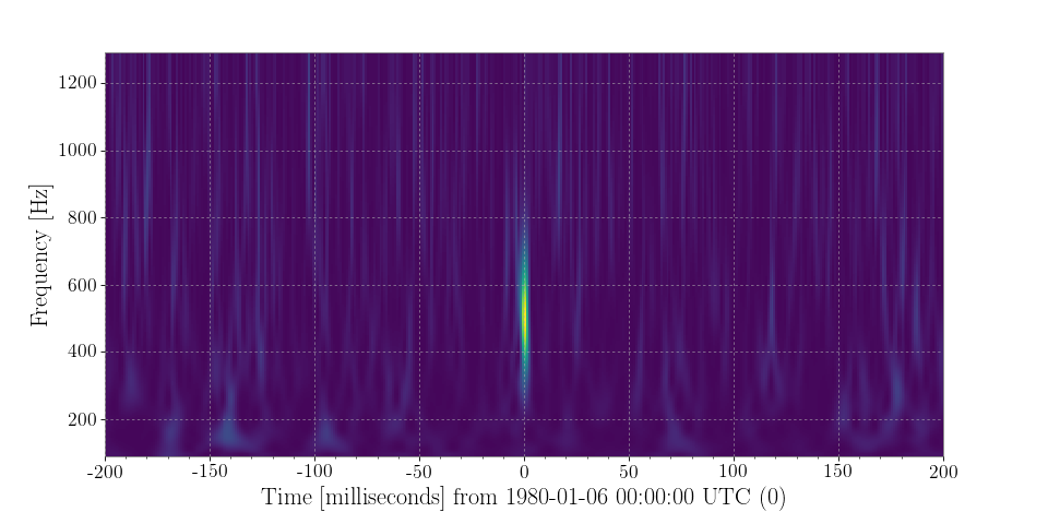
>>> from numpy.random import normal
>>> from scipy.signal import gausspulse
>>> from gwpy.timeseries import TimeSeries

Generate a TimeSeries containing Gaussian noise sampled at 4096 Hz, centred on GPS time 0, with a sine-Gaussian pulse (‘glitch’) at 500 Hz:

>>> noise = TimeSeries(normal(loc=1, size=4096*4), sample_rate=4096, epoch=-2)
>>> glitch = TimeSeries(gausspulse(noise.times.value, fc=500) * 4, sample_rate=4096)
>>> data = noise + glitch

Compute and plot the Q-transform of these data:

>>> q = data.q_transform()
>>> plot = q.plot()
>>> ax = plot.gca()
>>> ax.set_xlim(-.2, .2)
>>> ax.set_epoch(0)
>>> plot.show()

(png)

ravel([order])¶

Return a flattened array.

Refer to numpy.ravel for full documentation.

See also

numpy.ravel

equivalent function

ndarray.flat

a flat iterator on the array.

rayleigh_spectrogram(stride, fftlength=None, overlap=0, nproc=1, **kwargs)[source]¶

Calculate the Rayleigh statistic spectrogram of this TimeSeries

Parameters:	stride : float number of seconds in single PSD (column of spectrogram). fftlength : float number of seconds in single FFT. overlap : float, optional number of seconds of overlap between FFTs, default: 0 nproc : int, optional maximum number of independent frame reading processes, default default: 1
Returns:	spectrogram : Spectrogram time-frequency Rayleigh spectrogram as generated from the input time-series.

rayleigh_spectrum(fftlength=None, overlap=None)[source]¶

Calculate the Rayleigh FrequencySeries for this TimeSeries.

Parameters:	fftlength : float number of seconds in single FFT, defaults to a single FFT covering the full duration overlap : float, optional number of seconds of overlap between FFTs, defaults to that of the relevant method.
Returns:	psd : FrequencySeries a data series containing the PSD.

read(source, *args, **kwargs)[source]¶

Read data into a TimeSeries

Arguments and keywords depend on the output format, see the online documentation for full details for each format, the parameters below are common to most formats.

Parameters:

source : str, Cache source of data, any of the following: str path of single data file str path of LAL-format cache file Cache describing one or more data files, name : str, Channel the name of the channel to read, or a Channel object. start : LIGOTimeGPS, float, str, optional GPS start time of required data, defaults to start of data found; any input parseable by to_gps is fine end : LIGOTimeGPS, float, str, optional GPS end time of required data, defaults to end of data found; any input parseable by to_gps is fine format : str, optional source format identifier. If not given, the format will be detected if possible. See below for list of acceptable formats. nproc : int, optional number of parallel processes to use, serial process by default. Note Parallel frame reading, via the nproc keyword argument, is only available when giving a Cache of frames, or using the format='cache' keyword argument. gap : str, optional how to handle gaps in the cache, one of ‘ignore’: do nothing, let the undelying reader method handle it ‘warn’: do nothing except print a warning to the screen ‘raise’: raise an exception upon finding a gap (default) ‘pad’: insert a value to fill the gaps pad : float, optional value with which to fill gaps in the source data, only used if gap is not given, or gap='pad' is given

Notes

The available built-in formats are:

Format	Read	Write	Auto-identify	Deprecated
ascii.losc	Yes	No	No
csv	Yes	Yes	Yes
framecpp	Yes	Yes	No
gwf	Yes	Yes	Yes
gwf.framecpp	Yes	Yes	No
gwf.lalframe	Yes	Yes	No
hdf5	Yes	Yes	Yes
hdf5.losc	Yes	No	No
lalframe	Yes	Yes	No
txt	Yes	Yes	Yes
wav	Yes	No	No
losc	Yes	No	No	Yes

Deprecated format names like aastex will be removed in a future version. Use the full name (e.g. ascii.aastex) instead.

repeat(repeats, axis=None)¶

Repeat elements of an array.

Refer to numpy.repeat for full documentation.

See also

numpy.repeat

equivalent function

resample(rate, window='hamming', ftype='fir', n=None)[source]¶

Resample this Series to a new rate

Parameters:

rate : float rate to which to resample this Series window : str, numpy.ndarray, optional window function to apply to signal in the Fourier domain, see scipy.signal.get_window() for details on acceptable formats, only used for ftype='fir' or irregular downsampling ftype : str, optional type of filter, either ‘fir’ or ‘iir’, defaults to ‘fir’ n : int, optional if ftype='fir' the number of taps in the filter, otherwise the order of the Chebyshev type I IIR filter

Returns:

Series a new Series with the resampling applied, and the same metadata

reshape(shape, order='C')¶

Returns an array containing the same data with a new shape.

Refer to numpy.reshape for full documentation.

See also

numpy.reshape

equivalent function

resize(new_shape, refcheck=True)¶

Change shape and size of array in-place.

Parameters:	new_shape : tuple of ints, or n ints Shape of resized array. refcheck : bool, optional If False, reference count will not be checked. Default is True.
Returns:	None
Raises:	ValueError If a does not own its own data or references or views to it exist, and the data memory must be changed. PyPy only: will always raise if the data memory must be changed, since there is no reliable way to determine if references or views to it exist. SystemError If the order keyword argument is specified. This behaviour is a bug in NumPy.

See also

resize

Return a new array with the specified shape.

Notes

This reallocates space for the data area if necessary.

Only contiguous arrays (data elements consecutive in memory) can be resized.

The purpose of the reference count check is to make sure you do not use this array as a buffer for another Python object and then reallocate the memory. However, reference counts can increase in other ways so if you are sure that you have not shared the memory for this array with another Python object, then you may safely set refcheck to False.

Examples

Shrinking an array: array is flattened (in the order that the data are stored in memory), resized, and reshaped:

>>> a = np.array([[0, 1], [2, 3]], order='C')
>>> a.resize((2, 1))
>>> a
array([[0],
       [1]])

>>> a = np.array([[0, 1], [2, 3]], order='F')
>>> a.resize((2, 1))
>>> a
array([[0],
       [2]])

Enlarging an array: as above, but missing entries are filled with zeros:

>>> b = np.array([[0, 1], [2, 3]])
>>> b.resize(2, 3) # new_shape parameter doesn't have to be a tuple
>>> b
array([[0, 1, 2],
       [3, 0, 0]])

Referencing an array prevents resizing…

>>> c = a
>>> a.resize((1, 1))
Traceback (most recent call last):
...
ValueError: cannot resize an array that has been referenced ...

Unless refcheck is False:

>>> a.resize((1, 1), refcheck=False)
>>> a
array([[0]])
>>> c
array([[0]])

rms(stride=1)[source]¶

Calculate the root-mean-square value of this TimeSeries once per stride.

Parameters:	stride : float stride (seconds) between RMS calculations
Returns:	rms : TimeSeries a new TimeSeries containing the RMS value with dt=stride

round(decimals=0, out=None)¶

Return a with each element rounded to the given number of decimals.

Refer to numpy.around for full documentation.

See also

numpy.around

equivalent function

searchsorted(v, side='left', sorter=None)¶

Find indices where elements of v should be inserted in a to maintain order.

For full documentation, see numpy.searchsorted

See also

numpy.searchsorted

equivalent function

setfield(val, dtype, offset=0)¶

Put a value into a specified place in a field defined by a data-type.

Place val into a’s field defined by dtype and beginning offset bytes into the field.

Parameters:	val : object Value to be placed in field. dtype : dtype object Data-type of the field in which to place val. offset : int, optional The number of bytes into the field at which to place val.
Returns:	None

See also

getfield

Examples

>>> x = np.eye(3)
>>> x.getfield(np.float64)
array([[ 1.,  0.,  0.],
       [ 0.,  1.,  0.],
       [ 0.,  0.,  1.]])
>>> x.setfield(3, np.int32)
>>> x.getfield(np.int32)
array([[3, 3, 3],
       [3, 3, 3],
       [3, 3, 3]])
>>> x
array([[  1.00000000e+000,   1.48219694e-323,   1.48219694e-323],
       [  1.48219694e-323,   1.00000000e+000,   1.48219694e-323],
       [  1.48219694e-323,   1.48219694e-323,   1.00000000e+000]])
>>> x.setfield(np.eye(3), np.int32)
>>> x
array([[ 1.,  0.,  0.],
       [ 0.,  1.,  0.],
       [ 0.,  0.,  1.]])

setflags(write=None, align=None, uic=None)¶

Set array flags WRITEABLE, ALIGNED, and UPDATEIFCOPY, respectively.

These Boolean-valued flags affect how numpy interprets the memory area used by a (see Notes below). The ALIGNED flag can only be set to True if the data is actually aligned according to the type. The UPDATEIFCOPY flag can never be set to True. The flag WRITEABLE can only be set to True if the array owns its own memory, or the ultimate owner of the memory exposes a writeable buffer interface, or is a string. (The exception for string is made so that unpickling can be done without copying memory.)

Parameters:	write : bool, optional Describes whether or not a can be written to. align : bool, optional Describes whether or not a is aligned properly for its type. uic : bool, optional Describes whether or not a is a copy of another “base” array.

Notes

Array flags provide information about how the memory area used for the array is to be interpreted. There are 6 Boolean flags in use, only three of which can be changed by the user: UPDATEIFCOPY, WRITEABLE, and ALIGNED.

WRITEABLE (W) the data area can be written to;

ALIGNED (A) the data and strides are aligned appropriately for the hardware (as determined by the compiler);

UPDATEIFCOPY (U) this array is a copy of some other array (referenced by .base). When this array is deallocated, the base array will be updated with the contents of this array.

All flags can be accessed using their first (upper case) letter as well as the full name.

Examples

>>> y
array([[3, 1, 7],
       [2, 0, 0],
       [8, 5, 9]])
>>> y.flags
  C_CONTIGUOUS : True
  F_CONTIGUOUS : False
  OWNDATA : True
  WRITEABLE : True
  ALIGNED : True
  UPDATEIFCOPY : False
>>> y.setflags(write=0, align=0)
>>> y.flags
  C_CONTIGUOUS : True
  F_CONTIGUOUS : False
  OWNDATA : True
  WRITEABLE : False
  ALIGNED : False
  UPDATEIFCOPY : False
>>> y.setflags(uic=1)
Traceback (most recent call last):
  File "<stdin>", line 1, in <module>
ValueError: cannot set UPDATEIFCOPY flag to True

shift(delta)[source]¶

Shift this TimeSeries forward in time by delta

This modifies the series in-place.

Parameters:	delta : float, Quantity, str The amount by which to shift (in seconds if float), give a negative value to shift backwards in time

Examples

>>> from gwpy.timeseries import TimeSeries
>>> a = TimeSeries([1, 2, 3, 4, 5], t0=0, dt=1)
>>> print(a.t0)
0.0 s
>>> a.shift(5)
>>> print(a.t0)
5.0 s
>>> a.shift('-1 hour')
-3595.0 s

sort(axis=-1, kind='quicksort', order=None)¶

Sort an array, in-place.

Parameters:

axis : int, optional Axis along which to sort. Default is -1, which means sort along the last axis. kind : {‘quicksort’, ‘mergesort’, ‘heapsort’}, optional Sorting algorithm. Default is ‘quicksort’. order : str or list of str, optional When a is an array with fields defined, this argument specifies which fields to compare first, second, etc. A single field can be specified as a string, and not all fields need be specified, but unspecified fields will still be used, in the order in which they come up in the dtype, to break ties.

See also

numpy.sort

Return a sorted copy of an array.

argsort

Indirect sort.

lexsort

Indirect stable sort on multiple keys.

searchsorted

Find elements in sorted array.

partition

Partial sort.

Notes

See sort for notes on the different sorting algorithms.

Examples

>>> a = np.array([[1,4], [3,1]])
>>> a.sort(axis=1)
>>> a
array([[1, 4],
       [1, 3]])
>>> a.sort(axis=0)
>>> a
array([[1, 3],
       [1, 4]])

Use the order keyword to specify a field to use when sorting a structured array:

>>> a = np.array([('a', 2), ('c', 1)], dtype=[('x', 'S1'), ('y', int)])
>>> a.sort(order='y')
>>> a
array([('c', 1), ('a', 2)],
      dtype=[('x', '|S1'), ('y', '<i4')])

spectral_variance(stride, fftlength=None, overlap=None, method='scipy-welch', window='hann', nproc=1, filter=None, bins=None, low=None, high=None, nbins=500, log=False, norm=False, density=False)[source]¶

Calculate the SpectralVariance of this TimeSeries.

Parameters:

stride : float number of seconds in single PSD (column of spectrogram) fftlength : float number of seconds in single FFT method : str, optional FFT-averaging method, default: 'scipy-welch', see Notes for more details overlap : float, optional number of seconds of overlap between FFTs, defaults to the recommended overlap for the given window (if given), or 0 window : str, numpy.ndarray, optional window function to apply to timeseries prior to FFT, see scipy.signal.get_window() for details on acceptable formats nproc : int maximum number of independent frame reading processes, default is set to single-process file reading. bins : numpy.ndarray, optional, default None array of histogram bin edges, including the rightmost edge low : float, optional left edge of lowest amplitude bin, only read if bins is not given high : float, optional right edge of highest amplitude bin, only read if bins is not given nbins : int, optional number of bins to generate, only read if bins is not given log : bool, optional calculate amplitude bins over a logarithmic scale, only read if bins is not given norm : bool, optional normalise bin counts to a unit sum density : bool, optional normalise bin counts to a unit integral

Returns:

specvar : SpectralVariance 2D-array of spectral frequency-amplitude counts

See also

numpy.histogram()

for details on specifying bins and weights

Notes

The available methods are:

Method name	Function
welch	gwpy.signal.fft.basic.welch
bartlett	gwpy.signal.fft.basic.bartlett
median	gwpy.signal.fft.basic.median
median_mean	gwpy.signal.fft.basic.median_mean
pycbc_welch	gwpy.signal.fft.pycbc.welch
pycbc_bartlett	gwpy.signal.fft.pycbc.bartlett
pycbc_median	gwpy.signal.fft.pycbc.median
pycbc_median_mean	gwpy.signal.fft.pycbc.median_mean
lal_welch	gwpy.signal.fft.lal.welch
lal_bartlett	gwpy.signal.fft.lal.bartlett
lal_median	gwpy.signal.fft.lal.median
lal_median_mean	gwpy.signal.fft.lal.median_mean
scipy_welch	gwpy.signal.fft.scipy.welch
scipy_bartlett	gwpy.signal.fft.scipy.bartlett

See FFT routines for GWpy for more details

spectrogram(stride, fftlength=None, overlap=None, window='hann', method='scipy-welch', nproc=1, **kwargs)[source]¶

Calculate the average power spectrogram of this TimeSeries using the specified average spectrum method.

Each time-bin of the output Spectrogram is calculated by taking a chunk of the TimeSeries in the segment [t - overlap/2., t + stride + overlap/2.) and calculating the psd() of those data.

As a result, each time-bin is calculated using stride + overlap seconds of data.

Parameters:

stride : float number of seconds in single PSD (column of spectrogram). fftlength : float number of seconds in single FFT. overlap : float, optional number of seconds of overlap between FFTs, defaults to the recommended overlap for the given window (if given), or 0 window : str, numpy.ndarray, optional window function to apply to timeseries prior to FFT, see scipy.signal.get_window() for details on acceptable formats method : str, optional FFT-averaging method, default: 'scipy-welch', see Notes for more details nproc : int number of CPUs to use in parallel processing of FFTs

Returns:

spectrogram : Spectrogram time-frequency power spectrogram as generated from the input time-series.

Notes

The available methods are:

Method name	Function
welch	gwpy.signal.fft.basic.welch
bartlett	gwpy.signal.fft.basic.bartlett
median	gwpy.signal.fft.basic.median
median_mean	gwpy.signal.fft.basic.median_mean
pycbc_welch	gwpy.signal.fft.pycbc.welch
pycbc_bartlett	gwpy.signal.fft.pycbc.bartlett
pycbc_median	gwpy.signal.fft.pycbc.median
pycbc_median_mean	gwpy.signal.fft.pycbc.median_mean
lal_welch	gwpy.signal.fft.lal.welch
lal_bartlett	gwpy.signal.fft.lal.bartlett
lal_median	gwpy.signal.fft.lal.median
lal_median_mean	gwpy.signal.fft.lal.median_mean
scipy_welch	gwpy.signal.fft.scipy.welch
scipy_bartlett	gwpy.signal.fft.scipy.bartlett

See FFT routines for GWpy for more details

spectrogram2(fftlength, overlap=0, **kwargs)[source]¶

Calculate the non-averaged power Spectrogram of this TimeSeries

Parameters:

fftlength : float number of seconds in single FFT. overlap : float, optional number of seconds of overlap between FFTs, defaults to the recommended overlap for the given window (if given), or 0 window : str, numpy.ndarray, optional window function to apply to timeseries prior to FFT, see scipy.signal.get_window() for details on acceptable formats scaling : [ ‘density’ | ‘spectrum’ ], optional selects between computing the power spectral density (‘density’) where the Spectrogram has units of V**2/Hz if the input is measured in V and computing the power spectrum (‘spectrum’) where the Spectrogram has units of V**2 if the input is measured in V. Defaults to ‘density’. **kwargs other parameters to be passed to scipy.signal.periodogram for each column of the Spectrogram

Returns:

spectrogram: `~gwpy.spectrogram.Spectrogram` a power Spectrogram with 1/fftlength frequency resolution and (fftlength - overlap) time resolution.

See also

scipy.signal.periodogram

for documentation on the Fourier methods used in this calculation

Notes

This method calculates overlapping periodograms for all possible chunks of data entirely containing within the span of the input TimeSeries, then normalises the power in overlapping chunks using a triangular window centred on that chunk which most overlaps the given Spectrogram time sample.

squeeze(axis=None)¶

Remove single-dimensional entries from the shape of a.

Refer to numpy.squeeze for full documentation.

See also

numpy.squeeze

equivalent function

std(axis=None, dtype=None, out=None, ddof=0, keepdims=False)¶

Returns the standard deviation of the array elements along given axis.

Refer to numpy.std for full documentation.

See also

numpy.std

equivalent function

sum(axis=None, dtype=None, out=None, keepdims=False)¶

Return the sum of the array elements over the given axis.

Refer to numpy.sum for full documentation.

See also

numpy.sum

equivalent function

swapaxes(axis1, axis2)¶

Return a view of the array with axis1 and axis2 interchanged.

Refer to numpy.swapaxes for full documentation.

See also

numpy.swapaxes

equivalent function

take(indices, axis=None, out=None, mode='raise')¶

Return an array formed from the elements of a at the given indices.

Refer to numpy.take for full documentation.

See also

numpy.take

equivalent function

to(unit, equivalencies=[])¶

Return a new Quantity object with the specified unit.

Parameters:

unit : UnitBase instance, str An object that represents the unit to convert to. Must be an UnitBase object or a string parseable by the units package. equivalencies : list of equivalence pairs, optional A list of equivalence pairs to try if the units are not directly convertible. See Equivalencies. If not provided or [], class default equivalencies will be used (none for Quantity, but may be set for subclasses) If None, no equivalencies will be applied at all, not even any set globally or within a context.

See also

to_value

get the numerical value in a given unit.

to_lal()[source]¶

Convert this TimeSeries into a LAL TimeSeries.

to_pycbc(copy=True)[source]¶

Convert this TimeSeries into a PyCBC TimeSeries

Parameters:	copy : bool, optional, default: True if True, copy these data to a new array
Returns:	timeseries : TimeSeries a PyCBC representation of this TimeSeries

to_value(unit=None, equivalencies=[])¶

The numerical value, possibly in a different unit.

Parameters:

unit : UnitBase instance or str, optional The unit in which the value should be given. If not given or None, use the current unit. equivalencies : list of equivalence pairs, optional A list of equivalence pairs to try if the units are not directly convertible (see Equivalencies). If not provided or [], class default equivalencies will be used (none for Quantity, but may be set for subclasses). If None, no equivalencies will be applied at all, not even any set globally or within a context.

Returns:

value : ndarray or scalar The value in the units specified. For arrays, this will be a view of the data if no unit conversion was necessary.

See also

to

Get a new instance in a different unit.

tobytes(order='C')¶

Construct Python bytes containing the raw data bytes in the array.

Constructs Python bytes showing a copy of the raw contents of data memory. The bytes object can be produced in either ‘C’ or ‘Fortran’, or ‘Any’ order (the default is ‘C’-order). ‘Any’ order means C-order unless the F_CONTIGUOUS flag in the array is set, in which case it means ‘Fortran’ order.

New in version 1.9.0.

Parameters:	order : {‘C’, ‘F’, None}, optional Order of the data for multidimensional arrays: C, Fortran, or the same as for the original array.
Returns:	s : bytes Python bytes exhibiting a copy of a’s raw data.

Examples

>>> x = np.array([[0, 1], [2, 3]])
>>> x.tobytes()
b'\x00\x00\x00\x00\x01\x00\x00\x00\x02\x00\x00\x00\x03\x00\x00\x00'
>>> x.tobytes('C') == x.tobytes()
True
>>> x.tobytes('F')
b'\x00\x00\x00\x00\x02\x00\x00\x00\x01\x00\x00\x00\x03\x00\x00\x00'

tofile(fid, sep="", format="%s")¶

Write array to a file as text or binary (default).

Data is always written in ‘C’ order, independent of the order of a. The data produced by this method can be recovered using the function fromfile().

Parameters:	fid : file or str An open file object, or a string containing a filename. sep : str Separator between array items for text output. If “” (empty), a binary file is written, equivalent to file.write(a.tobytes()). format : str Format string for text file output. Each entry in the array is formatted to text by first converting it to the closest Python type, and then using “format” % item.

Notes

This is a convenience function for quick storage of array data. Information on endianness and precision is lost, so this method is not a good choice for files intended to archive data or transport data between machines with different endianness. Some of these problems can be overcome by outputting the data as text files, at the expense of speed and file size.

tolist()¶

Return the array as a (possibly nested) list.

Return a copy of the array data as a (nested) Python list. Data items are converted to the nearest compatible Python type.

Parameters:	none
Returns:	y : list The possibly nested list of array elements.

Notes

The array may be recreated, a = np.array(a.tolist()).

Examples

>>> a = np.array([1, 2])
>>> a.tolist()
[1, 2]
>>> a = np.array([[1, 2], [3, 4]])
>>> list(a)
[array([1, 2]), array([3, 4])]
>>> a.tolist()
[[1, 2], [3, 4]]

tostring(order='C')[source]¶

Construct Python bytes containing the raw data bytes in the array.

Constructs Python bytes showing a copy of the raw contents of data memory. The bytes object can be produced in either ‘C’ or ‘Fortran’, or ‘Any’ order (the default is ‘C’-order). ‘Any’ order means C-order unless the F_CONTIGUOUS flag in the array is set, in which case it means ‘Fortran’ order.

This function is a compatibility alias for tobytes. Despite its name it returns bytes not strings.

Parameters:	order : {‘C’, ‘F’, None}, optional Order of the data for multidimensional arrays: C, Fortran, or the same as for the original array.
Returns:	s : bytes Python bytes exhibiting a copy of a’s raw data.

Examples

>>> x = np.array([[0, 1], [2, 3]])
>>> x.tobytes()
b'\x00\x00\x00\x00\x01\x00\x00\x00\x02\x00\x00\x00\x03\x00\x00\x00'
>>> x.tobytes('C') == x.tobytes()
True
>>> x.tobytes('F')
b'\x00\x00\x00\x00\x02\x00\x00\x00\x01\x00\x00\x00\x03\x00\x00\x00'

trace(offset=0, axis1=0, axis2=1, dtype=None, out=None)¶

Return the sum along diagonals of the array.

Refer to numpy.trace for full documentation.

See also

numpy.trace

equivalent function

transpose(*axes)¶

Returns a view of the array with axes transposed.

For a 1-D array, this has no effect. (To change between column and row vectors, first cast the 1-D array into a matrix object.) For a 2-D array, this is the usual matrix transpose. For an n-D array, if axes are given, their order indicates how the axes are permuted (see Examples). If axes are not provided and a.shape = (i[0], i[1], ... i[n-2], i[n-1]), then a.transpose().shape = (i[n-1], i[n-2], ... i[1], i[0]).

Parameters:	axes : None, tuple of ints, or n ints None or no argument: reverses the order of the axes. tuple of ints: i in the j-th place in the tuple means a’s i-th axis becomes a.transpose()’s j-th axis. n ints: same as an n-tuple of the same ints (this form is intended simply as a “convenience” alternative to the tuple form)
Returns:	out : ndarray View of a, with axes suitably permuted.

See also

ndarray.T

Array property returning the array transposed.

Examples

>>> a = np.array([[1, 2], [3, 4]])
>>> a
array([[1, 2],
       [3, 4]])
>>> a.transpose()
array([[1, 3],
       [2, 4]])
>>> a.transpose((1, 0))
array([[1, 3],
       [2, 4]])
>>> a.transpose(1, 0)
array([[1, 3],
       [2, 4]])

update(other, inplace=True)[source]¶

Update this series by appending new data from an other and dropping the same amount of data off the start.

This is a convenience method that just calls append with resize=False.

value_at(x)[source]¶

Return the value of this Series at the given xindex value

Parameters:	x : float, Quantity the xindex value at which to search
Returns:	y : Quantity the value of this Series at the given xindex value

var(axis=None, dtype=None, out=None, ddof=0, keepdims=False)¶

Returns the variance of the array elements, along given axis.

Refer to numpy.var for full documentation.

See also

numpy.var

equivalent function

view(dtype=None, type=None)¶

New view of array with the same data.

Parameters:

dtype : data-type or ndarray sub-class, optional Data-type descriptor of the returned view, e.g., float32 or int16. The default, None, results in the view having the same data-type as a. This argument can also be specified as an ndarray sub-class, which then specifies the type of the returned object (this is equivalent to setting the type parameter). type : Python type, optional Type of the returned view, e.g., ndarray or matrix. Again, the default None results in type preservation.

Notes

a.view() is used two different ways:

a.view(some_dtype) or a.view(dtype=some_dtype) constructs a view of the array’s memory with a different data-type. This can cause a reinterpretation of the bytes of memory.

a.view(ndarray_subclass) or a.view(type=ndarray_subclass) just returns an instance of ndarray_subclass that looks at the same array (same shape, dtype, etc.) This does not cause a reinterpretation of the memory.

For a.view(some_dtype), if some_dtype has a different number of bytes per entry than the previous dtype (for example, converting a regular array to a structured array), then the behavior of the view cannot be predicted just from the superficial appearance of a (shown by print(a)). It also depends on exactly how a is stored in memory. Therefore if a is C-ordered versus fortran-ordered, versus defined as a slice or transpose, etc., the view may give different results.

Examples

>>> x = np.array([(1, 2)], dtype=[('a', np.int8), ('b', np.int8)])

Viewing array data using a different type and dtype:

>>> y = x.view(dtype=np.int16, type=np.matrix)
>>> y
matrix([[513]], dtype=int16)
>>> print(type(y))
<class 'numpy.matrixlib.defmatrix.matrix'>

Creating a view on a structured array so it can be used in calculations

>>> x = np.array([(1, 2),(3,4)], dtype=[('a', np.int8), ('b', np.int8)])
>>> xv = x.view(dtype=np.int8).reshape(-1,2)
>>> xv
array([[1, 2],
       [3, 4]], dtype=int8)
>>> xv.mean(0)
array([ 2.,  3.])

Making changes to the view changes the underlying array

>>> xv[0,1] = 20
>>> print(x)
[(1, 20) (3, 4)]

Using a view to convert an array to a recarray:

>>> z = x.view(np.recarray)
>>> z.a
array([1], dtype=int8)

Views share data:

>>> x[0] = (9, 10)
>>> z[0]
(9, 10)

Views that change the dtype size (bytes per entry) should normally be avoided on arrays defined by slices, transposes, fortran-ordering, etc.:

>>> x = np.array([[1,2,3],[4,5,6]], dtype=np.int16)
>>> y = x[:, 0:2]
>>> y
array([[1, 2],
       [4, 5]], dtype=int16)
>>> y.view(dtype=[('width', np.int16), ('length', np.int16)])
Traceback (most recent call last):
  File "<stdin>", line 1, in <module>
ValueError: new type not compatible with array.
>>> z = y.copy()
>>> z.view(dtype=[('width', np.int16), ('length', np.int16)])
array([[(1, 2)],
       [(4, 5)]], dtype=[('width', '<i2'), ('length', '<i2')])

whiten(fftlength, overlap=0, method='scipy-welch', window='hanning', detrend='constant', asd=None, **kwargs)[source]¶

White this TimeSeries against its own ASD

Parameters:

fftlength : float number of seconds in single FFT overlap : float, optional number of seconds of overlap between FFTs, defaults to the recommended overlap for the given window (if given), or 0 method : str, optional FFT-averaging method, default: 'scipy-welch', see Notes for more details window : str, numpy.ndarray, optional window function to apply to timeseries prior to FFT, see scipy.signal.get_window() for details on acceptable formats detrend : str, optional type of detrending to do before FFT (see detrend for more details) asd : FrequencySeries the amplitude-spectral density using which to whiten the data **kwargs other keyword arguments are passed to the TimeSeries.asd method to estimate the amplitude spectral density FrequencySeries of this TimeSeries

Returns:

out : TimeSeries a whitened version of the input data

See also

TimeSeries.asd

for details on the ASD calculation

numpy.fft

for details on the Fourier transform algorithm used her

scipy.signal

write(target, *args, **kwargs)[source]¶

Write this TimeSeries to a file

Parameters:	target : str path of output file format : str, optional output format identifier. If not given, the format will be detected if possible. See below for list of acceptable formats.

Notes

The available built-in formats are:

Format	Read	Write	Auto-identify
csv	Yes	Yes	Yes
framecpp	Yes	Yes	No
gwf	Yes	Yes	Yes
gwf.framecpp	Yes	Yes	No
gwf.lalframe	Yes	Yes	No
hdf5	Yes	Yes	Yes
lalframe	Yes	Yes	No
txt	Yes	Yes	Yes
wav	Yes	Yes	No

zip()[source]¶

Zip the xindex and value arrays of this Series

Returns:	stacked : 2-d numpy.ndarray The array formed by stacking the the xindex and value of this series

Examples

>>> a = Series([0, 2, 4, 6, 8], xindex=[-5, -4, -3, -2, -1])
>>> a.zip()
array([[-5.,  0.],
       [-4.,  2.],
       [-3.,  4.],
       [-2.,  6.],
       [-1.,  8.]])

zpk(zeros, poles, gain, analog=True, **kwargs)[source]¶

Filter this TimeSeries by applying a zero-pole-gain filter

Parameters:	zeros : array-like list of zero frequencies (in Hertz) poles : array-like list of pole frequencies (in Hertz) gain : float DC gain of filter analog : bool, optional type of ZPK being applied, if analog=True all parameters will be converted in the Z-domain for digital filtering
Returns:	timeseries : TimeSeries the filtered version of the input data

See also

TimeSeries.filter

for details on how a digital ZPK-format filter is applied

Examples

To apply a zpk filter with file poles at 100 Hz, and five zeros at 1 Hz (giving an overall DC gain of 1e-10):

>>> data2 = data.zpk([100]*5, [1]*5, 1e-10)

DictClass[source]¶

alias of TimeSeriesDict

asd(fftlength=None, overlap=None, window='hann', method='scipy-welch', **kwargs)[source]

Calculate the ASD FrequencySeries of this TimeSeries

Parameters:

fftlength : float number of seconds in single FFT, defaults to a single FFT covering the full duration overlap : float, optional number of seconds of overlap between FFTs, defaults to the recommended overlap for the given window (if given), or 0 window : str, numpy.ndarray, optional window function to apply to timeseries prior to FFT, see scipy.signal.get_window() for details on acceptable formats method : str, optional FFT-averaging method, default: 'scipy-welch', see Notes for more details

Returns:

psd : FrequencySeries a data series containing the PSD.

See also

TimeSeries.psd

Notes

The available methods are:

Method name	Function
welch	gwpy.signal.fft.basic.welch
bartlett	gwpy.signal.fft.basic.bartlett
median	gwpy.signal.fft.basic.median
median_mean	gwpy.signal.fft.basic.median_mean
pycbc_welch	gwpy.signal.fft.pycbc.welch
pycbc_bartlett	gwpy.signal.fft.pycbc.bartlett
pycbc_median	gwpy.signal.fft.pycbc.median
pycbc_median_mean	gwpy.signal.fft.pycbc.median_mean
lal_welch	gwpy.signal.fft.lal.welch
lal_bartlett	gwpy.signal.fft.lal.bartlett
lal_median	gwpy.signal.fft.lal.median
lal_median_mean	gwpy.signal.fft.lal.median_mean
scipy_welch	gwpy.signal.fft.scipy.welch
scipy_bartlett	gwpy.signal.fft.scipy.bartlett

See FFT routines for GWpy for more details

auto_coherence(dt, fftlength=None, overlap=None, window='hann', **kwargs)[source]

Calculate the frequency-coherence between this TimeSeries and a time-shifted copy of itself.

The standard TimeSeries.coherence() is calculated between the input TimeSeries and a cropped copy of itself. Since the cropped version will be shorter, the input series will be shortened to match.

Parameters:

dt : float duration (in seconds) of time-shift fftlength : float, optional number of seconds in single FFT, defaults to a single FFT covering the full duration overlap : float, optional number of seconds of overlap between FFTs, defaults to the recommended overlap for the given window (if given), or 0 window : str, numpy.ndarray, optional window function to apply to timeseries prior to FFT, see scipy.signal.get_window() for details on acceptable formats **kwargs any other keyword arguments accepted by matplotlib.mlab.cohere() except NFFT, window, and noverlap which are superceded by the above keyword arguments

Returns:

coherence : FrequencySeries the coherence FrequencySeries of this TimeSeries with the other

See also

matplotlib.mlab.cohere()

for details of the coherence calculator

Notes

The TimeSeries.auto_coherence() will perform best when dt is approximately fftlength / 2.

average_fft(fftlength=None, overlap=0, window=None)[source]

Compute the averaged one-dimensional DFT of this TimeSeries.

This method computes a number of FFTs of duration fftlength and overlap (both given in seconds), and returns the mean average. This method is analogous to the Welch average method for power spectra.

Parameters:	fftlength : float number of seconds in single FFT, default, use whole TimeSeries overlap : float, optional number of seconds of overlap between FFTs, defaults to the recommended overlap for the given window (if given), or 0 window : str, numpy.ndarray, optional window function to apply to timeseries prior to FFT, see scipy.signal.get_window() for details on acceptable formats
Returns:	out : complex-valued FrequencySeries the transformed output, with populated frequencies array metadata

See also

scipy.fftpack, used.

bandpass(flow, fhigh, gpass=2, gstop=30, fstop=None, type='iir', filtfilt=True, **kwargs)[source]

Filter this TimeSeries with a band-pass filter.

Parameters:

flow : float lower corner frequency of pass band fhigh : float upper corner frequency of pass band gpass : float the maximum loss in the passband (dB). gstop : float the minimum attenuation in the stopband (dB). fstop : tuple of float, optional (low, high) edge-frequencies of stop band type : str the filter type, either 'iir' or 'fir' **kwargs other keyword arguments are passed to gwpy.signal.filter_design.bandpass()

Returns:

bpseries : TimeSeries a band-passed version of the input TimeSeries

See also

gwpy.signal.filter_design.bandpass

for details on the filter design

TimeSeries.filter

for details on how the filter is applied

When using scipy < 0.16.0 some higher-order filters may be unstable. With scipy >= 0.16.0 higher-order filters are decomposed into second-order-sections, and so are much more stable.

coherence(other, fftlength=None, overlap=None, window='hann', **kwargs)[source]

Calculate the frequency-coherence between this TimeSeries and another.

Parameters:

other : TimeSeries TimeSeries signal to calculate coherence with fftlength : float, optional number of seconds in single FFT, defaults to a single FFT covering the full duration overlap : float, optional number of seconds of overlap between FFTs, defaults to the recommended overlap for the given window (if given), or 0 window : str, numpy.ndarray, optional window function to apply to timeseries prior to FFT, see scipy.signal.get_window() for details on acceptable formats **kwargs any other keyword arguments accepted by matplotlib.mlab.cohere() except NFFT, window, and noverlap which are superceded by the above keyword arguments

Returns:

coherence : FrequencySeries the coherence FrequencySeries of this TimeSeries with the other

See also

matplotlib.mlab.cohere()

for details of the coherence calculator

Notes

If self and other have difference TimeSeries.sample_rate values, the higher sampled TimeSeries will be down-sampled to match the lower.

coherence_spectrogram(other, stride, fftlength=None, overlap=None, window='hann', nproc=1)[source]

Calculate the coherence spectrogram between this TimeSeries and other.

Parameters:

other : TimeSeries the second TimeSeries in this CSD calculation stride : float number of seconds in single PSD (column of spectrogram) fftlength : float number of seconds in single FFT overlap : float, optional number of seconds of overlap between FFTs, defaults to the recommended overlap for the given window (if given), or 0 window : str, numpy.ndarray, optional window function to apply to timeseries prior to FFT, see scipy.signal.get_window() for details on acceptable formats nproc : int number of parallel processes to use when calculating individual coherence spectra.

Returns:

spectrogram : Spectrogram time-frequency coherence spectrogram as generated from the input time-series.

csd(other, fftlength=None, overlap=None, window='hann', **kwargs)[source]

Calculate the CSD FrequencySeries for two TimeSeries

Parameters:

other : TimeSeries the second TimeSeries in this CSD calculation fftlength : float number of seconds in single FFT, defaults to a single FFT covering the full duration overlap : float, optional number of seconds of overlap between FFTs, defaults to the recommended overlap for the given window (if given), or 0 window : str, numpy.ndarray, optional window function to apply to timeseries prior to FFT, see scipy.signal.get_window() for details on acceptable formats

Returns:

csd : FrequencySeries a data series containing the CSD.

csd_spectrogram(other, stride, fftlength=None, overlap=0, window='hann', nproc=1, **kwargs)[source]

Calculate the cross spectral density spectrogram of this

TimeSeries with ‘other’.

Parameters:

other : TimeSeries second time-series for cross spectral density calculation stride : float number of seconds in single PSD (column of spectrogram). fftlength : float number of seconds in single FFT. overlap : float, optional number of seconds of overlap between FFTs, defaults to the recommended overlap for the given window (if given), or 0 window : str, numpy.ndarray, optional window function to apply to timeseries prior to FFT, see scipy.signal.get_window() for details on acceptable formats nproc : int maximum number of independent frame reading processes, default is set to single-process file reading.

Returns:

spectrogram : Spectrogram time-frequency cross spectrogram as generated from the two input time-series.

demodulate(f, stride=1, exp=False, deg=True)[source]

Compute the average magnitude and phase of this TimeSeries

once per stride at a given frequency.

Parameters:	f : float frequency (Hz) at which to demodulate the signal stride : float, optional stride (seconds) between calculations, defaults to 1 second exp : bool, optional return the demodulated magnitude and phase trends as one TimeSeries object representing a complex exponential deg : bool, optional if exp=False, calculates the phase in degrees
Returns:	mag, phase : TimeSeries if exp=False, returns a pair of TimeSeries objects representing magnitude and phase trends with dt=stride out : TimeSeries if exp=True, returns a single TimeSeries with magnitude and phase trends represented as mag * exp(1j*phase) with dt=stride

Examples

Demodulation is useful when trying to examine steady sinusoidal signals we know to be contained within data. For instance, we can download some data from LOSC to look at trends of the amplitude and phase of Livingston’s calibration line at 331.3 Hz:

>>> from gwpy.timeseries import TimeSeries
>>> data = TimeSeries.fetch_open_data('L1', 1131350417, 1131357617)

We can demodulate the TimeSeries at 331.3 Hz with a stride of once per minute:

>>> amp, phase = data.demodulate(331.3, stride=60)

We can then plot these trends to visualize changes in the amplitude and phase of the calibration line:

>>> from gwpy.plotter import TimeSeriesPlot
>>> plot = TimeSeriesPlot(amp, phase, sep=True)
>>> plot.show()

(png)

detrend(detrend='constant')[source]

Remove the trend from this TimeSeries

This method just wraps scipy.signal.detrend() to return an object of the same type as the input.

Parameters:	detrend : str, optional the type of detrending.
Returns:	detrended : TimeSeries the detrended input series

See also

scipy.signal.detrend

for details on the options for the detrend argument, and how the operation is done

fft(nfft=None)[source]

Compute the one-dimensional discrete Fourier transform of this TimeSeries.

Parameters:	nfft : int, optional length of the desired Fourier transform, input will be cropped or padded to match the desired length. If nfft is not given, the length of the TimeSeries will be used
Returns:	out : FrequencySeries the normalised, complex-valued FFT FrequencySeries.

See also

scipy.fftpack, used.

Notes

This method, in constrast to the numpy.fft.rfft() method it calls, applies the necessary normalisation such that the amplitude of the output FrequencySeries is correct.

fftgram(stride)[source]

Calculate the Fourier-gram of this TimeSeries.

At every stride, a single, complex FFT is calculated.

Parameters:	stride : float number of seconds in single PSD (column of spectrogram)
Returns:	fftgram : Spectrogram a Fourier-gram

filter(*filt, **kwargs)[source]

Filter this TimeSeries with an IIR or FIR filter

Parameters:	*filt : filter arguments 1, 2, 3, or 4 arguments defining the filter to be applied, an Nx1 ndarray of FIR coefficients an Nx6 ndarray of SOS coefficients (numerator, denominator) polynomials (zeros, poles, gain) (A, B, C, D) ‘state-space’ representation filtfilt : bool, optional filter forward and backwards to preserve phase, default: False analog : bool, optional if True, filter coefficients will be converted from Hz to Z-domain digital representation, default: False inplace : bool, optional if True, this array will be overwritten with the filtered version, default: False **kwargs other keyword arguments are passed to the filter method
Returns:	result : TimeSeries the filtered version of the input TimeSeries
Raises:	ValueError if filt arguments cannot be interpreted properly

See also

scipy.signal.sosfilt

for details on filtering with second-order sections (scipy >= 0.16 only)

scipy.signal.sosfiltfilt

for details on forward-backward filtering with second-order sections (scipy >= 0.16 only)

scipy.signal.lfilter

for details on filtering (without SOS)

scipy.signal.filtfilt

for details on forward-backward filtering (without SOS)

Notes

IIR filters are converted either into cascading second-order sections (if scipy >= 0.16 is installed), or into the (numerator, denominator) representation before being applied to this TimeSeries.

Note

When using scipy < 0.16 some higher-order filters may be unstable. With scipy >= 0.16 higher-order filters are decomposed into second-order-sections, and so are much more stable.

FIR filters are passed directly to scipy.signal.lfilter() or scipy.signal.filtfilt() without any conversions.

Examples

We can design an arbitrarily complicated filter using gwpy.signal.filter_design

>>> from gwpy.signal import filter_design
>>> bp = filter_design.bandpass(50, 250, 4096.)
>>> notches = [filter_design.notch(f, 4096.) for f in (60, 120, 180)]
>>> zpk = filter_design.concatenate_zpks(bp, *notches)

And then can download some data from LOSC to apply it using TimeSeries.filter:

>>> from gwpy.timeseries import TimeSeries
>>> data = TimeSeries.fetch_open_data('H1', 1126259446, 1126259478)
>>> filtered = data.filter(zpk, filtfilt=True)

We can plot the original signal, and the filtered version, cutting off either end of the filtered data to remove filter-edge artefacts

>>> from gwpy.plotter import TimeSeriesPlot
>>> plot = TimeSeriesPlot(data, filtered[128:-128], sep=True)
>>> plot.show()

(png)

highpass(frequency, gpass=2, gstop=30, fstop=None, type='iir', filtfilt=True, **kwargs)[source]

Filter this TimeSeries with a high-pass filter.

Parameters:	frequency : float high-pass corner frequency gpass : float the maximum loss in the passband (dB). gstop : float the minimum attenuation in the stopband (dB). fstop : float stop-band edge frequency, defaults to frequency * 1.5 type : str the filter type, either 'iir' or 'fir' **kwargs other keyword arguments are passed to gwpy.signal.filter_design.highpass()
Returns:	hpseries : TimeSeries a high-passed version of the input TimeSeries

See also

gwpy.signal.filter_design.highpass

for details on the filter design

TimeSeries.filter

for details on how the filter is applied

When using scipy < 0.16.0 some higher-order filters may be unstable. With scipy >= 0.16.0 higher-order filters are decomposed into second-order-sections, and so are much more stable.

lowpass(frequency, gpass=2, gstop=30, fstop=None, type='iir', filtfilt=True, **kwargs)[source]

Filter this TimeSeries with a Butterworth low-pass filter.

Parameters:	frequency : float low-pass corner frequency gpass : float the maximum loss in the passband (dB). gstop : float the minimum attenuation in the stopband (dB). fstop : float stop-band edge frequency, defaults to frequency * 1.5 type : str the filter type, either 'iir' or 'fir' **kwargs other keyword arguments are passed to gwpy.signal.filter_design.lowpass()
Returns:	lpseries : TimeSeries a low-passed version of the input TimeSeries

See also

gwpy.signal.filter_design.lowpass

for details on the filter design

TimeSeries.filter

for details on how the filter is applied

When using scipy < 0.16.0 some higher-order filters may be unstable. With scipy >= 0.16.0 higher-order filters are decomposed into second-order-sections, and so are much more stable.

notch(frequency, type='iir', filtfilt=True, **kwargs)[source]

Notch out a frequency in this TimeSeries.

Parameters:	frequency : float, Quantity frequency (default in Hertz) at which to apply the notch type : str, optional type of filter to apply, currently only ‘iir’ is supported **kwargs other keyword arguments to pass to scipy.signal.iirdesign
Returns:	notched : TimeSeries a notch-filtered copy of the input TimeSeries

See also

TimeSeries.filter

for details on the filtering method

scipy.signal.iirdesign

for details on the IIR filter design method

psd(fftlength=None, overlap=None, window='hann', method='scipy-welch', **kwargs)[source]

Calculate the PSD FrequencySeries for this TimeSeries

Parameters:

fftlength : float number of seconds in single FFT, defaults to a single FFT covering the full duration overlap : float, optional number of seconds of overlap between FFTs, defaults to the recommended overlap for the given window (if given), or 0 window : str, numpy.ndarray, optional window function to apply to timeseries prior to FFT, see scipy.signal.get_window() for details on acceptable formats method : str, optional FFT-averaging method, default: 'scipy-welch', see Notes for more details **kwargs other keyword arguments are passed to the underlying PSD-generation method

Returns:

psd : FrequencySeries a data series containing the PSD.

Notes

The available methods are:

Method name	Function
welch	gwpy.signal.fft.basic.welch
bartlett	gwpy.signal.fft.basic.bartlett
median	gwpy.signal.fft.basic.median
median_mean	gwpy.signal.fft.basic.median_mean
pycbc_welch	gwpy.signal.fft.pycbc.welch
pycbc_bartlett	gwpy.signal.fft.pycbc.bartlett
pycbc_median	gwpy.signal.fft.pycbc.median
pycbc_median_mean	gwpy.signal.fft.pycbc.median_mean
lal_welch	gwpy.signal.fft.lal.welch
lal_bartlett	gwpy.signal.fft.lal.bartlett
lal_median	gwpy.signal.fft.lal.median
lal_median_mean	gwpy.signal.fft.lal.median_mean
scipy_welch	gwpy.signal.fft.scipy.welch
scipy_bartlett	gwpy.signal.fft.scipy.bartlett

See FFT routines for GWpy for more details

q_transform(qrange=(4, 64), frange=(0, inf), gps=None, search=0.5, tres=0.001, fres=0.5, norm='median', outseg=None, whiten=True, **asd_kw)[source]

Scan a TimeSeries using a multi-Q transform

Parameters:

qrange : tuple of float, optional (low, high) range of Qs to scan frange : tuple of float, optional (log, high) range of frequencies to scan gps : float, optional central time of interest for determine loudest Q-plane search : float, optional window around gps in which to find peak energies, only used if gps is given tres : float, optional desired time resolution (seconds) of output Spectrogram fres : float, None, optional desired frequency resolution (Hertz) of output Spectrogram, give None to skip this step and return the original resolution, e.g. if you’re going to do your own interpolation norm : bool, str, optional whether to normalize the returned Q-transform output, or how, default: True ('median'), other options: False, 'mean' outseg : Segment, optional GPS [start, stop) segment for output Spectrogram whiten : bool, FrequencySeries, optional boolean switch to enable (True) or disable (False) data whitening, or an ASD FrequencySeries with which to whiten the data **asd_kw keyword arguments to pass to TimeSeries.asd to generate an ASD to use when whitening the data

Returns:

specgram : Spectrogram output Spectrogram of normalised Q energy

See also

TimeSeries.asd

for documentation on acceptable **asd_kw

TimeSeries.whiten

for documentation on how the whitening is done

gwpy.signal.qtransform

for code and documentation on how the Q-transform is implemented

scipy.interpolate

for details on how the interpolation is implemented. This method uses InterpolatedUnivariateSpline to cast all frequency rows to the same time-axis, and then interpd to apply the desired frequency resolution across the band.

Notes

It is highly recommended to use the outseg keyword argument when only a small window around a given GPS time is of interest. This will speed up this method a little, but can greatly speed up rendering the resulting Spectrogram using pcolormesh.

If you aren’t going to use pcolormesh in the end, don’t worry.

Examples

>>> from numpy.random import normal
>>> from scipy.signal import gausspulse
>>> from gwpy.timeseries import TimeSeries

Generate a TimeSeries containing Gaussian noise sampled at 4096 Hz, centred on GPS time 0, with a sine-Gaussian pulse (‘glitch’) at 500 Hz:

>>> noise = TimeSeries(normal(loc=1, size=4096*4), sample_rate=4096, epoch=-2)
>>> glitch = TimeSeries(gausspulse(noise.times.value, fc=500) * 4, sample_rate=4096)
>>> data = noise + glitch

Compute and plot the Q-transform of these data:

>>> q = data.q_transform()
>>> plot = q.plot()
>>> ax = plot.gca()
>>> ax.set_xlim(-.2, .2)
>>> ax.set_epoch(0)
>>> plot.show()

(png)

rayleigh_spectrogram(stride, fftlength=None, overlap=0, nproc=1, **kwargs)[source]

Calculate the Rayleigh statistic spectrogram of this TimeSeries

Parameters:	stride : float number of seconds in single PSD (column of spectrogram). fftlength : float number of seconds in single FFT. overlap : float, optional number of seconds of overlap between FFTs, default: 0 nproc : int, optional maximum number of independent frame reading processes, default default: 1
Returns:	spectrogram : Spectrogram time-frequency Rayleigh spectrogram as generated from the input time-series.

rayleigh_spectrum(fftlength=None, overlap=None)[source]

Calculate the Rayleigh FrequencySeries for this TimeSeries.

Parameters:	fftlength : float number of seconds in single FFT, defaults to a single FFT covering the full duration overlap : float, optional number of seconds of overlap between FFTs, defaults to that of the relevant method.
Returns:	psd : FrequencySeries a data series containing the PSD.

resample(rate, window='hamming', ftype='fir', n=None)[source]

Resample this Series to a new rate

Parameters:

rate : float rate to which to resample this Series window : str, numpy.ndarray, optional window function to apply to signal in the Fourier domain, see scipy.signal.get_window() for details on acceptable formats, only used for ftype='fir' or irregular downsampling ftype : str, optional type of filter, either ‘fir’ or ‘iir’, defaults to ‘fir’ n : int, optional if ftype='fir' the number of taps in the filter, otherwise the order of the Chebyshev type I IIR filter

Returns:

Series a new Series with the resampling applied, and the same metadata

rms(stride=1)[source]

Calculate the root-mean-square value of this TimeSeries once per stride.

Parameters:	stride : float stride (seconds) between RMS calculations
Returns:	rms : TimeSeries a new TimeSeries containing the RMS value with dt=stride

spectral_variance(stride, fftlength=None, overlap=None, method='scipy-welch', window='hann', nproc=1, filter=None, bins=None, low=None, high=None, nbins=500, log=False, norm=False, density=False)[source]

Calculate the SpectralVariance of this TimeSeries.

Parameters:

stride : float number of seconds in single PSD (column of spectrogram) fftlength : float number of seconds in single FFT method : str, optional FFT-averaging method, default: 'scipy-welch', see Notes for more details overlap : float, optional number of seconds of overlap between FFTs, defaults to the recommended overlap for the given window (if given), or 0 window : str, numpy.ndarray, optional window function to apply to timeseries prior to FFT, see scipy.signal.get_window() for details on acceptable formats nproc : int maximum number of independent frame reading processes, default is set to single-process file reading. bins : numpy.ndarray, optional, default None array of histogram bin edges, including the rightmost edge low : float, optional left edge of lowest amplitude bin, only read if bins is not given high : float, optional right edge of highest amplitude bin, only read if bins is not given nbins : int, optional number of bins to generate, only read if bins is not given log : bool, optional calculate amplitude bins over a logarithmic scale, only read if bins is not given norm : bool, optional normalise bin counts to a unit sum density : bool, optional normalise bin counts to a unit integral

Returns:

specvar : SpectralVariance 2D-array of spectral frequency-amplitude counts

See also

numpy.histogram()

for details on specifying bins and weights

Notes

The available methods are:

Method name	Function
welch	gwpy.signal.fft.basic.welch
bartlett	gwpy.signal.fft.basic.bartlett
median	gwpy.signal.fft.basic.median
median_mean	gwpy.signal.fft.basic.median_mean
pycbc_welch	gwpy.signal.fft.pycbc.welch
pycbc_bartlett	gwpy.signal.fft.pycbc.bartlett
pycbc_median	gwpy.signal.fft.pycbc.median
pycbc_median_mean	gwpy.signal.fft.pycbc.median_mean
lal_welch	gwpy.signal.fft.lal.welch
lal_bartlett	gwpy.signal.fft.lal.bartlett
lal_median	gwpy.signal.fft.lal.median
lal_median_mean	gwpy.signal.fft.lal.median_mean
scipy_welch	gwpy.signal.fft.scipy.welch
scipy_bartlett	gwpy.signal.fft.scipy.bartlett

See FFT routines for GWpy for more details

spectrogram(stride, fftlength=None, overlap=None, window='hann', method='scipy-welch', nproc=1, **kwargs)[source]

Calculate the average power spectrogram of this TimeSeries using the specified average spectrum method.

Each time-bin of the output Spectrogram is calculated by taking a chunk of the TimeSeries in the segment [t - overlap/2., t + stride + overlap/2.) and calculating the psd() of those data.

As a result, each time-bin is calculated using stride + overlap seconds of data.

Parameters:

stride : float number of seconds in single PSD (column of spectrogram). fftlength : float number of seconds in single FFT. overlap : float, optional number of seconds of overlap between FFTs, defaults to the recommended overlap for the given window (if given), or 0 window : str, numpy.ndarray, optional window function to apply to timeseries prior to FFT, see scipy.signal.get_window() for details on acceptable formats method : str, optional FFT-averaging method, default: 'scipy-welch', see Notes for more details nproc : int number of CPUs to use in parallel processing of FFTs

Returns:

spectrogram : Spectrogram time-frequency power spectrogram as generated from the input time-series.

Notes

The available methods are:

Method name	Function
welch	gwpy.signal.fft.basic.welch
bartlett	gwpy.signal.fft.basic.bartlett
median	gwpy.signal.fft.basic.median
median_mean	gwpy.signal.fft.basic.median_mean
pycbc_welch	gwpy.signal.fft.pycbc.welch
pycbc_bartlett	gwpy.signal.fft.pycbc.bartlett
pycbc_median	gwpy.signal.fft.pycbc.median
pycbc_median_mean	gwpy.signal.fft.pycbc.median_mean
lal_welch	gwpy.signal.fft.lal.welch
lal_bartlett	gwpy.signal.fft.lal.bartlett
lal_median	gwpy.signal.fft.lal.median
lal_median_mean	gwpy.signal.fft.lal.median_mean
scipy_welch	gwpy.signal.fft.scipy.welch
scipy_bartlett	gwpy.signal.fft.scipy.bartlett

See FFT routines for GWpy for more details

spectrogram2(fftlength, overlap=0, **kwargs)[source]

Calculate the non-averaged power Spectrogram of this TimeSeries

Parameters:

fftlength : float number of seconds in single FFT. overlap : float, optional number of seconds of overlap between FFTs, defaults to the recommended overlap for the given window (if given), or 0 window : str, numpy.ndarray, optional window function to apply to timeseries prior to FFT, see scipy.signal.get_window() for details on acceptable formats scaling : [ ‘density’ | ‘spectrum’ ], optional selects between computing the power spectral density (‘density’) where the Spectrogram has units of V**2/Hz if the input is measured in V and computing the power spectrum (‘spectrum’) where the Spectrogram has units of V**2 if the input is measured in V. Defaults to ‘density’. **kwargs other parameters to be passed to scipy.signal.periodogram for each column of the Spectrogram

Returns:

spectrogram: `~gwpy.spectrogram.Spectrogram` a power Spectrogram with 1/fftlength frequency resolution and (fftlength - overlap) time resolution.

See also

scipy.signal.periodogram

for documentation on the Fourier methods used in this calculation

Notes

This method calculates overlapping periodograms for all possible chunks of data entirely containing within the span of the input TimeSeries, then normalises the power in overlapping chunks using a triangular window centred on that chunk which most overlaps the given Spectrogram time sample.

whiten(fftlength, overlap=0, method='scipy-welch', window='hanning', detrend='constant', asd=None, **kwargs)[source]

White this TimeSeries against its own ASD

Parameters:

fftlength : float number of seconds in single FFT overlap : float, optional number of seconds of overlap between FFTs, defaults to the recommended overlap for the given window (if given), or 0 method : str, optional FFT-averaging method, default: 'scipy-welch', see Notes for more details window : str, numpy.ndarray, optional window function to apply to timeseries prior to FFT, see scipy.signal.get_window() for details on acceptable formats detrend : str, optional type of detrending to do before FFT (see detrend for more details) asd : FrequencySeries the amplitude-spectral density using which to whiten the data **kwargs other keyword arguments are passed to the TimeSeries.asd method to estimate the amplitude spectral density FrequencySeries of this TimeSeries

Returns:

out : TimeSeries a whitened version of the input data

See also

TimeSeries.asd

for details on the ASD calculation

numpy.fft

for details on the Fourier transform algorithm used her

scipy.signal

zpk(zeros, poles, gain, analog=True, **kwargs)[source]

Filter this TimeSeries by applying a zero-pole-gain filter

Parameters:	zeros : array-like list of zero frequencies (in Hertz) poles : array-like list of pole frequencies (in Hertz) gain : float DC gain of filter analog : bool, optional type of ZPK being applied, if analog=True all parameters will be converted in the Z-domain for digital filtering
Returns:	timeseries : TimeSeries the filtered version of the input data

See also

TimeSeries.filter

for details on how a digital ZPK-format filter is applied

Examples

To apply a zpk filter with file poles at 100 Hz, and five zeros at 1 Hz (giving an overall DC gain of 1e-10):

>>> data2 = data.zpk([100]*5, [1]*5, 1e-10)
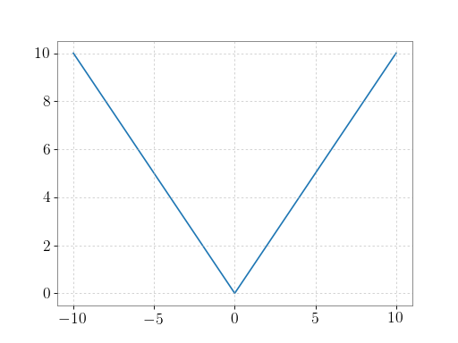
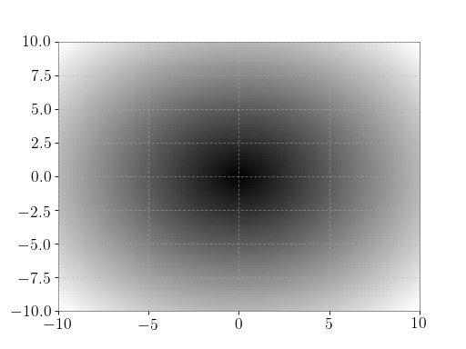
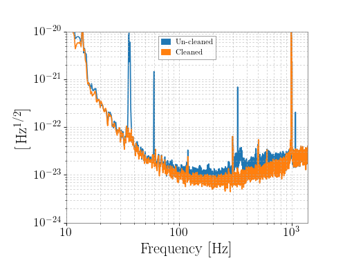
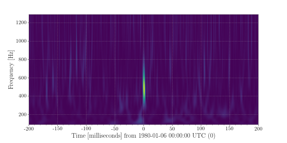