6. Generate the Q-transform of a TimeSeries
One of the most useful tools for filtering and visualising short-duration
features in a TimeSeries is the
Q-transform.
This is regularly used by the Detector Characterization working groups of
the LIGO Scientific Collaboration and the Virgo Collaboration to produce
high-resolution time-frequency maps of transient noise (glitches) and
potential gravitational-wave signals.
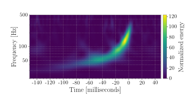
This algorithm was used to visualise the first ever gravitational-wave detection GW150914, so we can reproduce that result (bottom panel of figure 1) here.
First, we need to download the TimeSeries record for the H1 strain
measurement from LOSC:
from gwpy.timeseries import TimeSeries
data = TimeSeries.fetch_open_data('H1', 1126259446, 1126259478)
Next, we generate the q_transform of these data:
qspecgram = data.q_transform()
Now, we can plot the resulting Spectrogram, focusing on a
specific window around the interesting time
Note
Using crop is highly recommended at
this stage because rendering the high-resolution spectrogram as it is
done here is very slow (for experts this is because we’re using
pcolormesh and not any sort of image
interpolation, mainly to support both linear and log scaling nicely)
gps = 1126259462.427
plot = qspecgram.crop(gps-.15, gps+.05).plot(figsize=[8, 4])
ax = plot.gca()
ax.set_epoch(gps)
ax.set_yscale('log')
ax.set_xlabel('Time [milliseconds]')
ax.set_ylim(20, 500)
ax.grid(True, axis='y', which='both')
plot.add_colorbar(cmap='viridis', label='Normalized energy')
plot.show()
(png)

Here we can clearly see the trace of a compact binary coalescence, specifically a binary black hole coalescence! For more details on this result, please see http://www.ligo.org/science/Publication-GW150914/.