4. Comparing seismic trends between LIGO sites¶

On Feb 13 2015 there was a massive earthquake in the Atlantic Ocean, that should have had an impact on LIGO operations, I’d like to find out.

First: we import the objects we need, one for getting the data:

from gwpy.timeseries import TimeSeriesDict

and one for plotting the data:

from gwpy.plotter import TimeSeriesPlot

Next we define the channels we want, namely the 0.03Hz-1Hz ground motion band-limited RMS channels (1-second average trends). We do this using string-replacement so we can substitute the interferometer prefix easily when we need to:

channels = [
    '%s:ISI-BS_ST1_SENSCOR_GND_STS_X_BLRMS_30M_100M.mean,s-trend',
    '%s:ISI-BS_ST1_SENSCOR_GND_STS_Y_BLRMS_30M_100M.mean,s-trend',
    '%s:ISI-BS_ST1_SENSCOR_GND_STS_Z_BLRMS_30M_100M.mean,s-trend',
]

At last we can get() 12 hours of data for each interferometer:

lho = TimeSeriesDict.get([c % 'H1' for c in channels],
                         'Feb 13 2015 16:00', 'Feb 14 2015 04:00')
llo = TimeSeriesDict.get([c % 'L1' for c in channels],
                         'Feb 13 2015 16:00', 'Feb 14 2015 04:00')

Next we can plot the data, with a separate Axes for each instrument:

plot = TimeSeriesPlot(lho, llo)
ax1, ax2 = plot.axes
for ifo, ax in zip(('Hanford', 'Livingston'), (ax1, ax2)):
    ax.legend(['X', 'Y', 'Z'])
    ax.set_yscale('log')
    ax.text(1.01, 0.5, ifo, ha='left', va='center', transform=ax.transAxes,
            fontsize=18)
ax1.set_ylabel('$1-3$\,Hz motion [nm/s]', y=-0.1)
ax2.set_ylabel('')
ax1.set_title('Magnitude 7.1 earthquake impact on LIGO')
plot.show()

(png)

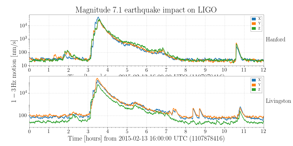
Here we have also customised the output by manually setting the legend entries, putting the interferometer label on the right-hand side, setting a logarithmic y-axis scale, adding a shared y-axis label on the left-hand side, and setting a title.

As we can see, the earthquake had a huge impact on the observatories, severly imparing operations for several hours.